Application and Implementation Examples of Directed Acyclic Graphs and Blockchain Technology

Introduction

Directed Acyclic Graph (DAG) is a graph data algorithm that appears in various situations such as automatic management of various tasks and compilers. In this article, I would like to discuss DAG.

Directed Acyclic Graphs

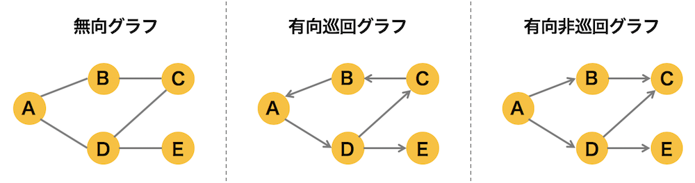
A Directed Acyclic Graph (DAG) is a type of directed graph that is not a “directed cyclic graph” with loops (cycles) on its path starting from any vertex, but one in which no loop exists. This means that if you start from a vertex and follow a directed edge, you will never pass through the same vertex more than once.

By taking advantage of these features, DAGs are used in a variety of applications, including the following

• Dependency Representation: DAGs are used to represent task and process dependencies. It is used to efficiently manage task execution order and dependencies by representing each task or process as a vertex and its dependencies as directed edges. Specifically, DAG is used to manage dependencies among source code and modules, data processing pipelines, and compilation processes in software development.
• Scheduling: DAGs are used to determine the order in which multiple tasks or jobs are executed. This is used, for example, in compilation and data flow programming, where each process, operation, or task is represented as a vertex and data dependencies are represented as directed edges to find the optimal order of execution.
• Program Flowchart: DAGs are sometimes used to graphically represent the control flow of a program. By representing conditional branches and loops as vertices and edges, the structure of the program can be easily understood visually.
• Compilation process: In the compilation of a programming language, source code is tokenized and parsed to construct a syntax tree. At this time, dependencies can be extracted as DAGs to obtain information for compilation order and optimization.
• Data analysis and machine learning: DAGs are used to represent data flows and computational graphs. In particular, DAGs can be used to represent computational graphs of machine learning models and algorithms, enabling efficient computation, automatic differentiation, and other advanced analysis methods. In big data processing and data pipelines, it is also common to represent data flows in DAGs, where each processing step or data stream is represented as a vertex and processing dependencies are represented as directed edges, which control data flow and processing order.

DAGs are data structures composed of a combination of vertices and edges, and can efficiently solve a variety of problems by taking advantage of their characteristics.

The details are described below.

Application Examples of Dependency Extraction by DAG

DAGs are widely used for dependency extraction and analysis, and their applications are described below.

• Software development projects: In software development, it is necessary to manage dependencies between source code and modules. By applying DAG to this, it is possible to determine the order of source code builds and tests, and to grasp the scope of influence of changes. Version control systems and dependency management tools (e.g., Maven and Gradle) also use DAG to resolve dependencies.
• Task Scheduling: DAGs are used to determine the order in which tasks and jobs are executed. This would be like, for example, a project management or workflow system where each task is represented as a vertex and dependencies as directed edges to effectively manage task execution order and dependencies.
• Data Processing Pipeline: In big data processing and data pipelines, it is common to represent the flow of data in a DAG. This is done by representing each processing step or data stream as a vertex and the processing dependencies as directed edges to control the flow of data and the order of processing.
• Compilation process: In compiling a programming language, source code is tokenized and parsed to construct a syntax tree. At this time, dependencies are extracted as DAGs to obtain information for compilation sequencing and optimization.

DAGs visualize the complexity of dependencies and can be a powerful tool for efficient parsing and determining the order in which tasks are executed.

Topological Sorting

<Overview>

Topological sort is an algorithm whose purpose is to order vertices in a DAG in the presence of dependencies from one vertex to another, in order to put them in the proper order.

Topological sort is mainly used to resolve the dependencies of tasks and events in a graph, which is applied, for example, in software build systems to resolve dependencies and to determine the order of execution of tasks in a project.

The procedure for topological sorting is as follows

1. Select a vertex with an in-degree of 0 and add it to the output column. The in-degree is the number of edges coming into a vertex.
2. Reduce the in-degree of the vertex adjacent to the selected vertex by 1. This means that one vertex dependent on the selected vertex has been resolved.
3. Select the vertex whose input degree has been reduced to zero, add it to the output column, and repeat.
4. Repeat steps 2-3 until there are no more vertices remaining in the graph.

If there are cycles (closed paths) in the graph, topological sorting cannot be performed because the dependencies among the vertices in the cycle are circular. Also, topological sorting can have a unique solution or multiple solutions. The unique solution is when the DAG has one connected component and the connected component is a directed tree (a special form of DAG), and the multiple solutions are when multiple nodes are at the same level (depth), This is the case when there are no dependencies between those nodes and the order can be swapped. Topological sort does not specify the order of nodes at the same level.

Topological Sort is an operation that arranges vertices in a linear order in a directed acyclic graph (DAG). This sort order is defined such that every edge in the graph comes before the vertex to which it points. In other words, to start from one vertex and reach another vertex, the other vertices must always be after that vertex.

Topological sorting is used to determine the order in which dependent tasks or processes are executed. Typical examples include software builds and task scheduling.

<Implementation in Python>

Below is an example implementation of topological sorting in Python.

from collections import defaultdict

def topological_sort(graph):
    # Array to manage vertex visit states
    visited = defaultdict(bool)
    # List to store topological sort results
    result = []

    # Function to perform depth-first search
    def dfs(node):
        visited[node] = True
        for neighbor in graph[node]:
            if not visited[neighbor]:
                dfs(neighbor)
        result.append(node)

    # Performs depth-first search using each vertex as a starting point
    for node in graph.keys():
        if not visited[node]:
            dfs(node)

    # Returns topological sort results with results in reverse order
    return result[::-1]

In this implementation, the graph is represented as a dictionary type, where the keys represent vertices, the value is a list of vertices ahead of the edge leaving that vertex, and the graph variable is passed this dictionary. topological_sort function performs topological sorting using depth-first search, the visited dictionary is used to sort each The visited state of each vertex is managed, the sorted vertices are added to the result list in reverse order, and finally, the result of the topological sort is returned with the result list in reverse order. The following is a running example.

# Definition of a directed acyclic graph (dictionary type)
graph = {
    'A': ['B', 'C'],
    'B': ['D'],
    'C': ['D', 'E'],
    'D': ['E'],
    'E': []
}

# Performing a topological sort
sorted_vertices = topological_sort(graph)

# Display Results
print(sorted_vertices)

In the above example, a topological sort is performed on the given graph and the results are displayed. The output is [‘A’, ‘C’, ‘E’, ‘D’, ‘B’].

Dijkstra’s algorithm and Bellman-Ford algorithm

<Overview>

Dijkstra’s algorithm (Dijkstra’s algorithm) and Bellman-Ford algorithm (Bellman-Ford algorithm) are algorithms for solving the shortest path problem in a graph. These algorithms can find the shortest path from one starting point to another by considering the weights of the vertices and edges of the graph.

Dijkstra’s method will be used to solve the single starting point shortest path problem, specifically, it will be the one that can find the shortest path in a directed graph with non-negative weights. The algorithm uses the method of selecting the vertex with the shortest distance from the starting vertex that has not been determined and updating the distances of the vertices directly connected from that vertex. This process is repeated until the shortest distance of all vertices is determined.

The Bellman-Ford method, on the other hand, is used to find the shortest path in a directed graph containing negative weights. The algorithm iteratively updates the set of vertices to see if a shorter path can be found. The Bellman-Ford method works for edges with negative weights, while the Dijkstra method does not give correct results for graphs with negative weights.

The main differences between the Dijkstra and Bellman-Ford methods will be the efficiency of the execution time and the restrictions on the graphs that can be handled. The Dijkstra method can quickly find the shortest path in graphs without negative weights, but it cannot obtain correct results in graphs with negative weights. On the other hand, the Bellman-Ford method works on graphs containing negative weights, but may require slower execution time.

<Implementation in Python>

Below are example implementations of the Dijkstra and Bellman-Ford methods in Python.

Example implementation of the Dijkstra method:

import heapq

def dijkstra(graph, start):
    distances = {node: float('inf') for node in graph}  # Initialize the distance of each node at infinity
    distances[start] = 0  # Set the distance of the starting point to 0
    queue = [(0, start)]  # A prioritized queue that stores tuples of (distance, node)

    while queue:
        current_distance, current_node = heapq.heappop(queue)  # Get the node with the minimum distance

        if current_distance > distances[current_node]:
            continue

        for neighbor, weight in graph[current_node].items():
            distance = current_distance + weight
            if distance < distances[neighbor]:
                distances[neighbor] = distance
                heapq.heappush(queue, (distance, neighbor))

    return distances

Usage example:.

graph = {
    'A': {'B': 5, 'C': 2},
    'B': {'D': 4, 'E': 2},
    'C': {'B': 8, 'E': 7},
    'D': {'E': 6, 'F': 3},
    'E': {'F': 1},
    'F': {}
}

start_node = 'A'
distances = dijkstra(graph, start_node)
print(distances)

Example implementation of the Bellman-Ford method:.

def bellman_ford(graph, start):
    distances = {node: float('inf') for node in graph}  # Initialize the distance of each node at infinity
    distances[start] = 0  # Set the distance of the starting point to 0

    for _ in range(len(graph) - 1):
        for node in graph:
            for neighbor, weight in graph[node].items():
                distance = distances[node] + weight
                if distance < distances[neighbor]:
                    distances[neighbor] = distance

    # Detection of negative weight cycles
    for node in graph:
        for neighbor, weight in graph[node].items():
            if distances[node] + weight < distances[neighbor]:
                raise ValueError("Negative weight cycles exist.")

    return distances

Usage example:.

graph = {
    'A': {'B': -1, 'C': 4},
    'B': {'C': 3, 'D': 2, 'E': 2},
    'C': {},
    'D': {'B': 1, 'C': 5},
    'E': {'D': -3}
}

start_node = 'A'
distances = bellman_ford(graph, start_node)
print(distances)

In the example implementation above, the graph is represented as a dictionary, where the weights of each node and its neighbors are stored in the form of a dictionary. The Dijkstra method uses a prioritized queue (heapq) to select nodes, while the Bellman-Ford method uses a double loop to update the shortest path.

Dynamic Programming

Dynamic Programming (Dynamic Programming) is a method for efficiently finding a solution to a complex problem by dividing it into smaller subproblems and saving and reusing the solution of each subproblem. Dynamic programming is a method of designing algorithms to solve problems using recursive relations and the principle of optimality.

The basic idea of dynamic programming is to use a property called “optimal substructure.” When the optimal solution consists of optimal solutions of multiple subproblems, the solution of each subproblem can be saved to avoid duplicate calculations and efficiently find a solution.

The general procedure of dynamic programming is as follows.

1. The problem is divided into smaller subproblems, and the subproblems are designed to avoid duplication.
2. The solutions to the subproblems are computed recursively or iteratively, and the computed solutions are memorized (stored).
3. To construct the final solution, the solutions of the subproblems are combined or the results are obtained recursively.

Dynamic programming can be applied to a variety of problems, including optimization, combinatorial, and shortest path problems. Typical examples of dynamic programming include computing the Fibonacci sequence and solving the knapsack problem.

The advantage of dynamic programming is that it can efficiently handle recursive relationships, and since the solution to a subproblem is memorized once calculated, recalculation is not required even if the same subproblem appears multiple times. However, since dynamic programming requires exhaustive solution of all subproblems, it may require exponential time and memory depending on the nature of the problem.

<Implementation of topological sorting using dynamic programming in python>

When topological sorting is performed using dynamic programming, the approach is to compute the topological sort order for each node, store it, and reuse it. The following is an example implementation of topological sorting using dynamic programming in Python.

def topological_sort(graph):
    # Dictionary to store the topological sort order of each node
    order = {}

    def dfs(node):
        if node in order:
            return order[node]

        max_order = 0
        for neighbor in graph[node]:
            neighbor_order = dfs(neighbor) + 1
            max_order = max(max_order, neighbor_order)

        order[node] = max_order
        return max_order

    # Run dfs on all nodes
    for node in graph:
        dfs(node)

    # Sort nodes in topological sort order
    sorted_nodes = sorted(graph, key=lambda x: order[x], reverse=True)
    return sorted_nodes

Usage example:.

graph = {
    'A': [],
    'B': ['A'],
    'C': ['A'],
    'D': ['B', 'C'],
    'E': ['D'],
    'F': ['D'],
    'G': ['E', 'F']
}

sorted_nodes = topological_sort(graph)
print(sorted_nodes)

In the above example implementation, the topological_sort function topologically sorts the given graph and returns a list of sorted nodes. Inside the function, the dfs function is called recursively to compute the topological sort order of each node and store it in the order dictionary. Finally, it sorts the nodes based on the order dictionary and returns a list of sorted nodes.

Strongly Connected Components

<Overview>

Strongly Connected Components decomposition is a method for partitioning a directed graph into smaller strongly connected components (sets of strongly connected vertices). Strongly Connected Components are collections of vertices that can reach each other and are characterized as substructures in the graph.

Strongly connected component decomposition is an important algorithm in directed graphs and has a variety of applications. It can be used, for example, in the analysis of dependencies in a graph or in compiler optimization.

The strongly connected component decomposition algorithm is usually performed in two phases: depth-first search (DFS) and search for inverse edge graphs. The following is the basic algorithmic procedure for strongly connected component decomposition.

1. For a given directed graph, a depth-first search (DFS) is performed. In this search, visit and end times are recorded for each vertex.
2. Reverse the orientation of all edges of the graph to create an inverse edge graph.
3. Perform a depth-first search (DFS) on the inverse edge graph in descending order of visit time. In this search, information on the strongly connected components belonging to each vertex is recorded.
4. The obtained set of strongly connected components is the result of strongly connected component decomposition.

<Implementation in Python>

The following is an example implementation of strongly connected component decomposition in Python (using Tarjan’s algorithm)

def tarjan_scc(graph):
    index_counter = [0]
    index = {}
    lowlink = {}
    on_stack = set()
    stack = []
    result = []

    def strongconnect(node):
        index[node] = index_counter[0]
        lowlink[node] = index_counter[0]
        index_counter[0] += 1
        stack.append(node)
        on_stack.add(node)

        for neighbor in graph[node]:
            if neighbor not in index:
                strongconnect(neighbor)
                lowlink[node] = min(lowlink[node], lowlink[neighbor])
            elif neighbor in on_stack:
                lowlink[node] = min(lowlink[node], index[neighbor])

        if lowlink[node] == index[node]:
            scc = []
            while True:
                w = stack.pop()
                on_stack.remove(w)
                scc.append(w)
                if w == node:
                    break
            result.append(scc)

    for node in graph:
        if node not in index:
            strongconnect(node)

    return result

Usage example:.

graph = {
    'A': ['B'],
    'B': ['C'],
    'C': ['A', 'D'],
    'D': ['E'],
    'E': ['F'],
    'F': ['D']
}

sccs = tarjan_scc(graph)
for scc in sccs:
    print(scc)

In the above example implementation, the tarjan_scc function performs strongly connected component decomposition of a given directed graph and uses Tarjan’s algorithm inside the function to find strongly connected components while performing depth-first search (DFS) and search for the inverse edge graph. Finally, a list of strongly connected components is returned. The execution results are as follows.

['E', 'F', 'D']
['C', 'B', 'A']

From this result, we find two strongly connected components in the graph, the first of which is ‘E’, ‘F’, and ‘D’, and the second of which is ‘C’, ‘B’, and ‘A’.

Finally, we discuss blockchain technology as it relates to DAGs.

Blockchain Technology and DAG

Blockchain technology and DAGs are both forms of distributed ledger technology, but with some important differences.

Blockchain records transaction history by grouping transactions into units called blocks and linking those blocks together. Each block refers to the hash value of the previous block and is connected as a chain. This concatenation of blocks is important to ensure the sequence and reliability of a series of transactions, and its main advantages are its high security and reliability. However, blockchains can pose challenges in scaling transactions because blocks are added sequentially.

A DAG, on the other hand, is not a linear chain like a blockchain, but rather a graph structure; in a DAG, transactions are not grouped into blocks, but rather individual transactions are connected by reference to each other. This connectivity allows for asynchronous approval of transactions, which is expected to increase throughput and improve scaling.

The main benefits of DAGs are network scaling and faster transactions. With DAGs, multiple transactions are processed simultaneously, reducing transaction approval times. Transaction fees may also be reduced.

However, DAGs also present some challenges. These include, for example, the risk of double payments and unauthorized manipulation because transaction sequencing is not guaranteed. It can also be difficult to design and secure DAGs.

In summary, blockchain focuses on transaction sequencing and reliability, while DAG is a technology that focuses on scaling and speed. Each technology has different advantages and challenges and should be selected according to the appropriate use case.

Reference Information and Reference Books

For more information on graph data handling, including DAGs, see “Graph Data Processing Algorithms and Applications to Machine Learning/Artificial Intelligence Tasks. See also here. Blockchain technology is also discussed in detail in “The Impact of Blockchain: A Disruptive Technology That Will Overhaul the Social Structure from Bitcoin, FinTech to IoT – A Note on Reading“.

A good reference book is “Graph Theory“.

“Graph Theory (Graduate Texts in Mathematics, 244)“

“Mastering Graph Data Structure in Python: From Theory to Practice: Unlocking the Power of Graph Data Structure in Python: From Fundamentals to Advanced Algorithms “

“Algorithms on Trees and Graphs: With Python Code“