
Overview of time series data analysis
Time-series data is called data whose values change over time, such as stock prices, temperatures, and traffic volumes. By applying machine learning to this time-series data, a large amount of data can be learned and used for business decision making and risk management by making predictions on unknown data.
Time-series data includes trends, seasonality, and random elements. Trends represent long-term trends, seasonality is cyclical patterns, and random elements are unpredictable noise. To take these factors into account, various methods are used in forecasting time-series data.
Among them, ARIMA described in “Examples of implementations for general time series analysis using R and Python”, Prophet described in “Time series analysis using Prophet“, LSTM described in “Overview of LSTM and Examples of Algorithms and Implementations“, and state-space models are representative methods used. These methods are prediction methods based on machine learning, which learns from past time-series data to predict the future.
Since time-series data includes time, in order to learn past data and predict the future, it is necessary to process the time-series data appropriately, for example, by decomposing the data into trend, seasonal, and residual components, which also requires various innovations.
In this article, we will focus on state-space models among these approaches.
The state space model
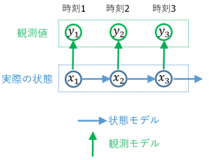
The state space model is one of the most commonly used stochastic models in time series analysis, incorporating observable variables, called observation variables, and unobservable variables, called state variables, as well as stochastic models to incorporate temporal variation and observation noise, and to represent the relationship between latent states and observed data The state-space model is a representation of the relationship between potential states and observed data. State-space models have a wide range of applications in signal processing, control engineering, economics, statistics, machine learning, and other fields.


The state-space model is expressed mathematically as follows
- State Equation: The state equation can be a difference or differential equation that shows how the potential state of the system changes with time. It is usually expressed as follows
\[y(t) = f(y(t-1), u(t-1), w(t))\]
Whereas、
-
- y(t) represents the state vector (internal state of the system) at time t,
- f is a function of the system’s equation of state, defining the system’s characteristics,
- u(t-1) represents the control input (external influence) at time t-1,
- w(t) represents random noise, called process noise, which represents unknown variations in the state equation.
- Observation Equation: The observation equation expresses how the observed data is generated from the state of the system. It is generally expressed as follows
\[x(t) = h(y(t), v(t))\]
Whereas、
-
- y(t) represents the observed data (usually from a sensor) at time t,
- h is a function representing the observation equation, which transforms the state vector x(t) into observed data,
- v(t) is the observation noise, a random variation that represents unknown noise in the observation equation.
- Initial State: The state-space model requires a value for the state vector x(0) at the initial time (t=0), which represents the initial conditions of the system.
- Properties of Noise:Process and observational noise usually assume a Gaussian (normal) distribution. Therefore, the state-space model is a probabilistic model as described in “Uncertainty and Machine Learning Techniques. If the noise follows a Gaussian distribution, it can be filtered and predicted using probabilistic estimation methods such as the Kalman filter. See also “Noise Removal, Data Cleansing, and Interpolation of Missing Values in Machine Learning” for details on handling noise.
Using these methods, state-space models typically use filtering (estimation of current state), prediction (estimation of future state), smoothing (estimation of past state), and other estimation methods to estimate the state of the system based on control inputs and observed data.
Algorithms used in state-space models
In state-space models, various algorithms are used to estimate states and model parameters. The main algorithms are described below.
- ARIMAmodel:
The ARIMA model, described in “Examples of implementations for general time series analysis using R and Python” is the model used when the state and observed variables follow a linear Gaussian distribution.
- Kalman Filter:
The Kalman filter, described in “State Space Models Using Clojure: Implementing the Kalman Filter” is a widely used algorithm for estimating state space models. The Kalman filter combines observed data, state equations, and models of the observed equations to perform real-time state estimation and prediction.
- Kalman Smoother:
The Kalman smoother is an algorithm that uses the results of the Kalman filter to modify past state estimates to produce a smoother state estimate. While the Kalman filter performs filtering (real-time) estimation, the Kalman smoother performs smoothing (modifying past estimates) estimation.
- Extended Kalman Filter:
The Kalman filter can be applied to linear models, but not directly to nonlinear models. Therefore, the extended Kalman filter (EKF) is used for nonlinear models; the EKF is a method of applying the Kalman filter by linearizing a nonlinear system in an approximate manner.
- Particle Filter:
The particle filter, also described in “Implementing Particle Filters on Time Series Data” is a Bayesian filtering technique that can be applied to nonlinear and non-Gaussian state-space models. This method uses random particles to approximate the probability distribution of states. It is a widely used alternative to the Kalman filter and EKF, especially for nonlinear and non-Gaussian models.
- Nonparametric Bayes:
Nonparametric Bayesian models, described in “Nonparametric Bayesian and Gaussian Processes” are used to solve nonlinear state-space models.
- Expectation-Maximization(EM) Algorithm:
The EM algorithm, described in “EM Algorithm and Examples of Various Application Implementations” is a method for estimating the parameters of a model that can simultaneously estimate the observed data and the hidden (unknown) state. It is particularly useful when there are missing data or when the state vector is not fully observable. See also “Noise Removal, Data Cleansing, and Missing Value Interpolation in Machine Learning” for more information on missing value completion.
Libraries and platforms used for state space models
State space models can be implemented using a variety of programming languages and numerical libraries. Below we describe some of the most commonly used libraries and platforms for implementing state-space models.
<Python>
- NumPy: A library for numerical computations, providing efficient processing of matrix operations, etc.
- SciPy: A library for scientific and technical computing, providing linear algebra, integration, optimization, signal processing, and other functions.
- Statsmodels: A library supporting statistical modeling, allowing estimation and prediction of state-space models.
- Kalman Filter Libraries: Libraries for implementing state estimation methods such as Kalman filters.
<R>
- dlm: A package to implement Dynamic Linear Models (DLM), which allows estimation of state space models and Kalman filters.
- KFAS: Kalman Filter and Smoother package, which enables state estimation by Kalman filter and smoother.
<MATLAB>
- System Identification Toolbox: A toolbox that identifies and estimates linear and nonlinear systems and can be used to estimate state-space models.
- Control System Toolbox: Provides functions related to control systems and supports state-space representation of control systems.
<Julia>
- DynamicalSystems.jl: This package will be dedicated to the analysis of dynamic systems, including the implementation of state-space models and Kalman filters.
The application of state-space models
State-space models have a wide range of applications in various fields. Some of the common applications of state-space models are listed below:
- Signal processing: State-space models are used in areas such as speech signal processing and image processing. For example, they are applied to speech signal denoising, speech recognition, and image tracking.
- Control Engineering: State space models are often used in the design and modeling of control systems. Algorithms such as Kalman filters and Kalman smoothers are used to achieve feedback and predictive control of control systems.
- Finance: State-space models are also applied in stock price forecasting and financial market modeling. They are used for estimating financial time series data, risk management, and portfolio optimization.
- Economics: State-space models are also used in economics to forecast economic indicators, analyze economic fluctuations, and evaluate fiscal policy.
- Robotics: In robotics, state-space models are used to estimate the posture and self-position of robots and to calibrate sensors.
- Biomedical: In the medical field, state-space models are used to analyze biological signals such as heart rate and blood pressure, and to model biological systems.
Beyond these, state-space models can be a powerful and flexible method for modeling time-series data and dynamic systems, and are a particularly useful approach when the data contains noise or unknown variability.
Finally, we will discuss an example implementation using python and R, which are the primary implementation methods.
Example implementation of analyzing time-series data with a state-space model using python
The statsmodels package is often used to analyze time series data using state-space models in Python. The following is a concrete implementation of the analysis of time series data with state-space models using the statsmodels package.
First, import the necessary libraries.
import numpy as np
import pandas as pd
import matplotlib.pyplot as plt
import statsmodels.api as sm
Next, time-series data is read in. Here, we use the time-series data of the number of passengers, AirPassengers.
# Loading Data
data = pd.read_csv("AirPassengers.csv", index_col=0, parse_dates=True)
Visualize the data.
# Data Visualization
plt.plot(data)
plt.xlabel("Year")
plt.ylabel("Passengers")
plt.show()
Next, a state-space model is constructed. Here, the ARIMA(1,1,1) model is used.
# Construction of state-space model
model = sm.tsa.statespace.SARIMAX(data, order=(1,1,1), seasonal_order=(0,0,0,0))
Estimate the state-space model.
# Estimation of state-space models
results = model.fit()
Confirm the results of the estimation.
# Display of estimation results
print(results.summary())
Finally, visualize the estimation results.
# Visualization of estimation results
results.plot_diagnostics()
plt.show()
Next, an example of analysis using R is described.
Example implementation of analyzing time-series data with a state-space model using R
In R, the stats package and the KFAS package can be used to analyze state-space models. Below is an example of analyzing time series data with a state-space model using the KFAS package.
As an example, assume the following AR(1) process.
\[y_t=\phi y_{t-1}+\epsilon_t,\ \epsilon_t\sim N(0,\sigma^2)\]
This AR(1) process is formulated as a state-space model and the parameters are estimated.
# Loading Data
data <- read.csv("data.csv")

# Loading the KFAS Package
library(KFAS)

# Defining the state space model
ss_model <- SSModel(formula = ~ -1 + AR1(phi = NA),
                    H = NA,
                    Q = diag(NA, 1),
                    data = data)

# Setting Initial Values
init_state <- c(y1 = data$y[1], phi = 0.5, sigma2 = var(data$y))

# Parameter Estimation by Maximum Likelihood Method
fit <- fitSSM(ss_model, inits = init_state)

# Display of estimated parameters
summary(fit)

# Display of state estimates and 95% confidence intervals
plot(states(fit), type = "l", main = "State Estimates with 95% CI")
abline(h = 0, col = "gray", lty = "dotted")
abline(h = c(-1.96, 1.96) * sqrt(fit$statesCov[, , 1]), col = "gray", lty = "dotted")
In this code, time series data are read from data.csv. Next, the state space model is defined by the SSModel function, and the parameters are estimated by the maximum likelihood method using the fitSSM function. Finally, the state estimates and 95% confidence intervals are plotted using the states and plot functions.
Reference Information and Reference Books
Time series data analysis is described in “Time Series Data Analysis.
General Introductions to State Space Models
-
“Time Series Analysis by State Space Methods” (2nd ed.) – James Durbin & Siem Jan Koopman (Oxford University Press, 2012)
-
A foundational text explaining state space representation, the Kalman filter, smoothing, and forecasting.
-
Includes worked examples (mostly in MATLAB, but concepts are directly transferable to R/Python).
-
-
“Dynamic Linear Models with R” – Giovanni Petris, Sonia Petrone & Patrizia Campagnoli (Springer, 2009)
-
Hands-on introduction using the
dlmpackage in R. -
Covers Bayesian state space modeling, filtering, and smoothing.
-
Applied and Computational Perspectives
-
“Applied Time Series Analysis” – Wayne A. Woodward, Henry L. Gray & Alan C. Elliott (CRC Press, 2017)
-
Covers classical and modern approaches including state space methods.
-
Provides R and some SAS code, but easily adapted to Python workflows.
-
-
“State-Space Methods for Time Series Analysis” – José Casals, Manuel J. Sotoca, Fernando Jareño & Anabel Ferrando (Springer, 2016)
-
Strong on theory with applied examples.
-
Offers computational recipes that can be implemented in R or Python.
-
Python & R Implementations
-
“Forecasting: Principles and Practice” (3rd ed., online) – Rob J Hyndman & George Athanasopoulos
-
Free online book, uses R (
forecast,fable,tsibble). -
While not exclusively about state space models, it introduces them in the context of exponential smoothing and ARIMA.
-
-
“Hands-On Time Series Analysis with R” – Rami Krispin (Packt, 2019)
-
Practical applications, including state space modeling via
forecast,bsts, andprophet.
-
-
“Applied Time Series Analysis with Python” – Aileen Nielsen (O’Reilly, 2019)
-
Focuses on practical implementation with Python’s
statsmodels,pmdarima, andpykalman. -
Includes examples of Kalman filtering and dynamic models.
-
-
“Bayesian Analysis of Time Series with Python” – Osvaldo Martin (Packt, 2021)
-
Demonstrates Bayesian state space modeling using PyMC3/PyMC4.
-
Useful for modern probabilistic programming approaches.
-
Reference book is “


“


“


“


AIシステム設計・意思決定構造の設計を専門としています。
Ontology・DSL・Behavior Treeによる判断の外部化、マルチエージェント構築に取り組んでいます。
Specialized in AI system design and decision-making architecture.
Focused on externalizing decision logic using Ontology, DSL, and Behavior Trees, and building multi-agent systems.


コメント