Implementation of hidden Markov model with Viterbi algorithm and stochastic generative model using Clojure
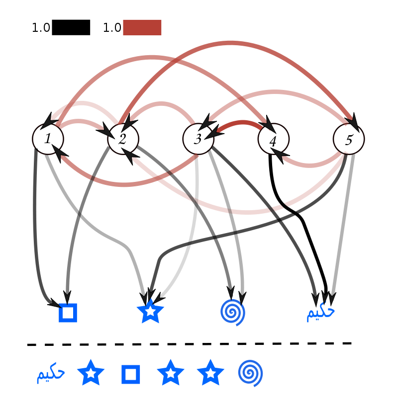
A hidden Markov model is a stochastic model, which is a Markov process with unobserved (hidden) states. Unlike a Markov process whose state is directly observable, a hidden Markov model uses information from observed data to infer the underlying “hidden” state. The figure below is an example of a hidden Markov model taken from the wiki page. The circles (1-5) at the top of the figure represent state transitions, and the symbols at the bottom represent observed information. When the actual observed information is the symbols shown in the lower part of the wavy line, there are three candidate state series that output them: “532532”, “432532”, and “312532”. Such a maximum likelihood observation series problem can be efficiently solved by the Viterbi algorithm described below.

Examples of concrete applications include methods that estimate hidden states for input information sequences with predefined meta-rules (state transitions) such as speech recognition, natural language, or processing of sensor information such as images and IOT, etc., by setting up hidden state transitions in advance, and combining these methods with BERT described in “BERT Overview, Algorithms, and Example Implementations“ There are various methods for inferring state transitions, such as those that combine these methods with BERT, etc., or those that combine them with probabilistic generative models such as nonparametric Bayesian models.
In this section, we first describe the Viterbi algorithm using Clojure. The module used is “clj-viterbi“. See “Getting Started with Clojure” for details on setting up the Clojure environment.
First, create a new project with “lein new viterbi-test (arbitrary project name)”. Add the library [com.lemonodor.viterbi “0.1.0”] to the project.clj file in the created project folder as follows.
(defproject viterbi-test "0.1.0-SNAPSHOT"
  :description "FIXME: write description"
  :url "http://example.com/FIXME"
  :license {:name "EPL-2.0 OR GPL-2.0-or-later WITH Classpath-exception-2.0"
            :url "https://www.eclipse.org/legal/epl-2.0/"}
  :dependencies [[org.clojure/clojure "1.11.1"]
                 [com.lemonodor.viterbi "0.1.0"]]
  :repl-options {:init-ns viterbi-test.core})
Next, define and evaluate the HMM in the core.clj file. The HMM to be defined this time is as follows.

The observed states are “Dizzy”, “Cold”, and “Normal”, and the hidden states are “Healthy” and “Fever”. The code for HMM using this is as follows.
(ns viterbi-test.core
  (:require [com.lemonodor.viterbi :as viterbi]))

(def hmm
  (viterbi/make-hmm
   :states [:healthy :fever]
   :start-p {:healthy 0.6, :fever 0.4}
   :trans-p (let [t {:healthy {:healthy 0.7, :fever 0.3},
                     :fever {:healthy 0.4, :fever 0.6}}]
              #((t %1) %2))
   :emit-p (let [t {:healthy {:normal 0.5, :cold 0.4, :dizzy 0.1},
                    :fever {:normal 0.1, :cold 0.3, :dizzy 0.6}}]
             #((t %1) %2))))
The :state variable sets the hidden state, the :start-p variable sets the respective initial probability (shown as probability from start in the above figure), the :trans-p variable sets the state transition probability of the hidden state, and the :emit-p variable defines the transition probability from the hidden state to the observed state.
These are evaluated as follows.
(viterbi/viterbi hmm [:normal :cold :dizzy])
;; -> [-1.8204482088348124 [:healthy :healthy :fever]]
The output data is the maximum likelihood estimated state transitions and their probabilities (log10-probability).
Next, we describe the HMM using anglican as described previously. Create a project file as described above, and add the library to the project.clj file.
(defproject hmm-test "0.1.0-SNAPSHOT"
  :description "FIXME: write description"
  :url "http://example.com/FIXME"
  :license {:name "EPL-2.0 OR GPL-2.0-or-later WITH Classpath-exception-2.0"
            :url "https://www.eclipse.org/legal/epl-2.0/"}
  :dependencies [[org.clojure/clojure "1.11.1"]
                 [anglican "1.1.0"]
                 [org.clojure/data.csv "1.0.1"]
                 [net.mikera/core.matrix "0.62.0"]
                 ;[plotly-clj "0.1.1"]
                 ;[org.nfrac/cljbox2d "0.5.0"]
                 ;[quil "3.1.0"]
                 ]
  :main ^:skip-aot gr-anglican.core
  :target-path "target/%s"
  :plugins [[org.clojars.benfb/lein-gorilla "0.6.0"]]
  :profiles {:uberjar {:aot :all
                       :jvm-opts ["-Dclojure.compiler.direct-linking=true"]}})
Next, the HMM model is described.
(ns hmm-test
  (:require [gorilla-plot.core :as plot]
            [clojure.core.matrix :as m]
            [anglican.stat :as s]
            :reload)
  (:use clojure.repl
        [anglican
          core runtime emit
          [inference :only [collect-by]]]))

(defn index->ind
  "converts a collection of indices to a matrix of indicator vectors"
  [values]
  (let [max-v (reduce max values)
        zero-vec (into [] (repeat (inc max-v) 0))]
    (m/matrix (map #(assoc zero-vec % 1) values))))

(defn square
  [x]
  (m/mul x x))
(defquery hmm
  "takes observation sequence and
  known initial state, transition,
  and observation distributions and
  returns posterior samples of the
  joint latent state sequence"
  [observations init-dist trans-dists obs-dists]
    (reduce
      (fn [states obs]
        (let [state (sample (get trans-dists
                                 (peek states)))]
          (observe (get obs-dists state) obs)
          (conj states state)))
      [(sample init-dist)]
      observations))
Describe the parameters. In this case, we will use 16 observation data and 3 state parameters.
(def data
  "observation sequence (16 points)"
  [0.9 0.8 0.7 0.0
   -0.025 -5.0 -2.0 -0.1
   0.0 0.13 0.45 6
   0.2 0.3 -1 -1])

(def init-dist
  "distribution on 0-th state in sequence
  (before first observation)"
  (discrete [1.0 1.0 1.0]))

(def trans-dists
  "transition distribution for each state"
  {0 (discrete [0.1 0.5 0.4])
   1 (discrete [0.2 0.2 0.6])
   2 (discrete [0.15 0.15 0.7])})

(def obs-dists
  "observation distribution for each state"
  {0 (normal -1 1)
   1 (normal 1 1)
   2 (normal 0 1)})
Perform inference using the Sequential Monte Carlo method
(def number-of-particles 1000)
(def number-of-samples 10000)

(def samples
  (->> (doquery :smc hmm
                [data
                 init-dist
                 trans-dists
                 obs-dists]
                :number-of-particles number-of-particles)
       (take number-of-samples)
       doall
       time))
Compare with the distribution calculated by the forward-backward method.
(def posterior
  "ground truth postior on states,
  calculated using forward-backwardi'm "
  [[ 0.3775 0.3092 0.3133]
   [ 0.0416 0.4045 0.5539]
   [ 0.0541 0.2552 0.6907]
   [ 0.0455 0.2301 0.7244]
   [ 0.1062 0.1217 0.7721]
   [ 0.0714 0.1732 0.7554]
   [ 0.9300 0.0001 0.0699]
   [ 0.4577 0.0452 0.4971]
   [ 0.0926 0.2169 0.6905]
   [ 0.1014 0.1359 0.7626]
   [ 0.0985 0.1575 0.744 ]
   [ 0.1781 0.2198 0.6022]
   [ 0.0000 0.9848 0.0152]
   [ 0.1130 0.1674 0.7195]
   [ 0.0557 0.1848 0.7595]
   [ 0.2017 0.0472 0.7511]
   [ 0.2545 0.0611 0.6844]])

(def num-sample-range (mapv (partial * number-of-samples)
                            [1e-2 2e-2 5e-2 1e-1 2e-1 5e-1 1]))
(def L2-errors
   (map (fn [n]
          (->> ;; use first n samples
               (take n samples)
               ;; calculate L2 error of empirical posterior relative to true posterior
               (collect-by (comp index->ind :result))
               s/empirical-mean
               (l2-norm posterior)))
        num-sample-range))

(plot/list-plot (map vector
                     (map #(/ (log %) (log 10)) num-sample-range)
                     (map #(/ (log %) (log 10)) L2-errors))
                :joined true
                :color "#05A"
                :x-title "log number of samples"
                :y-title "log L2 error")
The results are as follows

As previously discussed in “The Difference between Hidden Markov Models and State Space Models and Parameter Estimation for State Space Models,” a state space model is obtained by making the states of a hidden Markov model continuous. The stochastic approach to the Kalman filter is described separately.

コメント