Summary
From Clojure for Data Science. In this article, we describe network analysis using Clojure, including width-first/depth-first search, shortest path search, minimum spanning tree, subgraphs, and connected components.
Introduction
A graph is simply a set of vertices connected by edges, and the simplicity of this abstraction means that graphs are everywhere. Graphs are valid models for a wide variety of structures, including the hyperlink structure of the Web, the physical structure of the Internet, roads, telecommunications, and social networks.
Thus, network analysis is not new, but it is becoming more common, especially with the rise of social network analysis; Google, Facebook, Twitter, LinkedIn, and others are mining user data through large-scale graph processing. Given the critical importance of targeted advertising in website monetization, there are significant financial rewards for companies that effectively infer the interests of Internet users.
For these algorithms for graph data, we have previously described C++ implementations of “basic algorithms for graph data (DFS, BFS, bipartite graph decision, shortest path problem, minimum global tree)” and “advanced graph algorithms (strongly connected component decomposition, DAG, 2-SAT, LCA)“. In this article, we will discuss the use of Clojure/loom.
In this article, we will discuss the principles of network analysis using publicly available Twitter data as a concrete example. Pattern matching techniques such as triangle counting are applied to find structures in the graph, and graph-wide processing algorithms such as label propagation and PageRank are applied to find network structures in the graph. Finally, we use these techniques to identify the interests of the Twitter community from its most influential members.
Analysis using Twitter data
As a first concrete example, we will use follower data from the Twitter social network. This data is provided as part of the Stanford Large Network Dataset Collection. For the data to be used, follow the “Socila networks” and “ego-Twitter” links on the aforementioned page, and use the two files “twitter.tar.gz” and “twitter_combined.txt.gz”.
For details on setting up the Clojure environment, see “Getting Started with Clojure (1)” etc. For details, please refer to “Setting up a Clojure development environment with SublimeText4, VS code and LightTable“.
First, create a project file with “lein new network-analysis-test (any project name)” and add the library to the project.clj file in the project folder as follows
(defproject network-analysys-test "0.1.0-SNAPSHOT"
  :description "FIXME: write description"
  :url "http://example.com/FIXME"
  :license {:name "EPL-2.0 OR GPL-2.0-or-later WITH Classpath-exception-2.0"
            :url "https://www.eclipse.org/legal/epl-2.0/"}
  :dependencies [[org.clojure/clojure "1.11.1"]
                 [aysylu/loom "1.0.2"]
                 [incanter "1.9.3"]
                 [t6/from-scala "0.3.0"]
                 [glittering "0.1.2"]
                 [gorillalabs/sparkling "3.2.1"]
                 [org.apache.spark/spark-core_2.11 "2.4.8"]
                 [org.apache.spark/spark-graphx_2.11 "2.4.8"]
                 [org.clojure/data.csv "1.0.1"]]
  :repl-options {:init-ns network-analysys-test.core})
Details of the libraries to be added are described below. First, store the downloaded data under the resource folder and perform a simple graph data conversion and visualization using loom.
(ns network-analysys-test.core
  (:require [clojure.data.csv :as csv]
            [clojure.java.io :as io]
            [clojure.string :as str]
            [loom
             [graph :as loom]
             [io :as lio]
             [alg-generic :as gen]
             [alg :as alg]
             [gen :as generate]
             [attr :as attr]
             [label :as label]]
           ))

(defn to-long [s]
  (Long/parseLong s))

(defn line->edge [line]
  (->> (str/split line #" ")
       (mapv to-long)))

(defn load-edges [file]
  (->> (io/resource file)
       (io/reader)
       (line-seq)
       (map line->edge)))
When the above code reads the twitter data, it is confirmed that the data is a pair of two nodes, as shown below.
(load-edges "twitter/98801140.edges")
(["100873813" "3829151"]
 ["35432131" "3829151"]
 ["100742942" "35432131"]
 ["35432131" "27475761"]
 ["27475761" "35432131"])
This is then converted into graphical data using loom and further visualized.
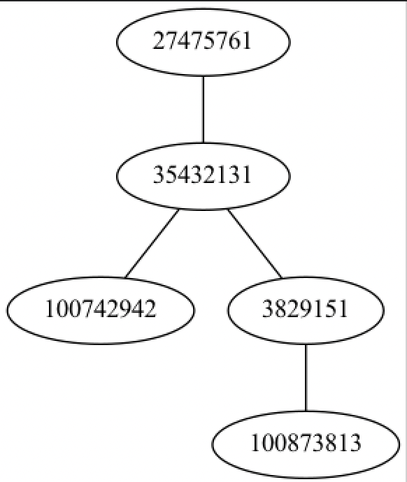
(->> (load-edges "twitter/98801140.edges")
     (apply loom/graph)
     (lio/view)))
loom/view requires graphviz, which must be installed beforehand (“brew install graphviz” for mac). The result will be a graph like the following.

Since there were five edges in the aforementioned data, but only four edges in the figure above, it is possible that this data is a directed graph. In that case, use the function “loom/diagraph” instead of “loom/graph
(defn testa5 [n]
  (->> (testa3 n)
       (apply loom/digraph)
       (lio/view)))

(testa5 "data/twitter/98801140.edges")
The results are shown below. It can be seen that the graph is a directed graph with five edges.

Since this data is from the twitter social graph, account 382951 has two followers, account 35432131 and 100873813, and there are two edges between account 27475761 and 35432131, forming a “cycle”. The two edges between accounts 27475761 and 35432131 form a “cycle”.
Exploring Graphs with Loom
The variety of phenomena that can be represented by graph models makes graph search algorithms very useful. For example, the Euler path on the Koenigsberg bridge (a path through all edges of the graph), described in “What is a complex network? This is a good thing. This is implemented as follows, and substituting the above graph yields the result “false”.
(defn euler-tour? [graph]
     (let [degree (partial loom/out-degree graph)]
       (->> (loom/nodes graph)
            (filter (comp odd? degree))
            (count)
            (contains? #{0 2}))))
(euler-tour?
   (->> (load-edges "twitter/98801140.edges")
        (apply loom/graph)))   ;; false
Width-first and depth-first search
A more common desire in graph search is to find nodes in a graph under certain constraints. There are several methods for this task; for unweighted graphs, such as the Twitter follow graph, the most common are width-first search and depth-first search.
Breadth-first search starts at a particular vertex and searches for vertices in its neighborhood. If that vertex is not found, the neighborhood is searched in turn until either the vertex is found or the entire graph is traversed.
The following figure shows the order in which vertices are searched, hierarchically from top to bottom, left to right.

Loom includes various search algorithms in the loom.alg namespace. Let’s run a width-first search on the same Twitter follower graph as before.
First, let’s look at width-first search. The width-first search is provided as a bf-traverse function. This function returns
The nodes visited by the width-first search are shown in order, and we can see how the width-first search traverses the graph.
(let [graph (->> (load-edges "twitter/98801140.edges")
                      (apply loom/digraph))]
       (alg/bf-traverse graph 100742942))

;;(100742942 35432131 27475761 3829151)
The above result uses the bf-traverse function to perform a traversal of the graph starting at node 100742942. The response does not include node 100873813. This indicates that there is no way to traverse the graph to this vertex by following the direction of the edge only. The only way to reach vertex 100742942 would be to start there.

Also, 35432131 is listed only once, even though it is connected to both 27475761 and 3829151; Loom’s implementation of width-first search keeps a set of visited vertices in memory, so once visited, it is not visited again.
An alternative to width-first search is depth-first search. This algorithm would proceed immediately to the bottom of the tree and visit the nodes in the order shown in the following figure.

The implementation in loom is as follows.
(let [graph (->> (load-edges "twitter/98801140.edges")
                      (apply loom/digraph))]
       (alg/pre-traverse graph 100742942))

;; (100742942 35432131 3829151 27475761)
The order of the nodes found is different from that of breadth-first search. The advantage of depth-first search is that it requires much less memory than breadth-first search because it does not need to store all nodes at each level. Thus, for large graphs, memory consumption may be lower.
However, in some situations, either depth-first or breadth-first search may be more convenient. For example, if you are looking for a living relative in a family tree, depth-first search may get you there faster because the person is likely to be at the bottom of the tree. If you are looking for an older ancestor, a depth-first search will check many newer relatives, and it will take much longer to reach your goal.
shortest path search
The aforementioned algorithms traversed the graph vertex by vertex and returned permutations of all nodes in the graph. While these are useful to illustrate the two primary ways to navigate the graph structure, the more general task is to find the shortest path from one vertex to another. In other words, we are interested only in the sequence of nodes in between.
For unweighted graphs, such as the one described above, distances are usually counted in terms of the number of “hops”. The shortest path will be the path with the fewest number of hops. In general, width-first search is a more efficient algorithm in this case.
Loom implements width-first shortest paths as bf-path functions. Their implementation is shown below. First, the following data is targeted.
(->> (load-edges "twitter/396721965.edges")
          (apply loom/digraph)
          (lio/view))
See if you can identify the shortest path between the upper and lower nodes 75914648 and 32122637. There are many possible paths that the algorithm could return. There are many possible paths that the algorithm could return, but here we want to identify the path through points 28719244 and 163629705. This will be the path with the fewest number of hops.
(let [graph (->> (load-edges "twitter/396721965.edges")
                      (apply loom/digraph))]
       (alg/bf-path graph 75914648 32122637))

;;(75914648 28719244 163629705 32122637)
It can be confirmed that those paths are actually extracted as shortest paths.
Loom also implements a bidirectional breadth-first shortest path algorithm called bf-path-bi. It performs parallel searches from both source and destination, and for certain types of graphs, it has the potential to find the shortest path faster.
Next we discuss the case where the graph has weights, this shortest hop may not correspond to the shortest path between two nodes. This is because this path may have a large weight. The algorithm to find them is the Dijkstra algorithm. This would be a method to find the shortest cost path between two nodes. This path may have a large number of hops, but the sum of the weights of the edges it passes through will be the smallest.
(let [graph (->> (load-edges "twitter/396721965.edges")
                      (apply loom/weighted-digraph))]
       (-> (loom/add-edges graph [28719244 163629705 100])
           (alg/dijkstra-path 75914648 32122637)))

;;(75914648 28719244 31477674 163629705 32122637)
The code reads the graph as a weighted graph and updates the weight of the edge between nodes 28719244 and 163629705 to 100. This has the effect of assigning a very high cost to the shortest path, allowing alternative paths to be found.
Dijkstra’s algorithm is particularly useful for path finding. For example, if the graph models a road network, a path through major roads may be more optimal than the shortest path. Also, the cost of a particular route may vary depending on the time of day and the amount of traffic on the road. In such cases, Dijkstra’s algorithm can determine the optimal route at any time of day.
Also called A* (pronounced A-star), the algorithm optimizes Dijkstra’s algorithm by allowing heuristic functions; it is implemented in Loom as alg/ astar-path. The heuristic function returns the expected cost to the destination. Any function can be used as a heuristic as long as it does not overestimate the true cost. By using this heuristic, the A* algorithm avoids an exhaustive search of the graph and thus
faster processing.
Minimum spanning tree
Next, we discuss the minimum spanning tree, an algorithm that discovers a path connecting all nodes in a graph. Minimum spanning trees can be thought of as a hybrid of the complete graph search algorithm and the shortest path algorithm described above.
Minimum spanning trees are particularly useful for weighted graphs. If the weights represent the cost of connecting two vertices, the minimum spanning tree finds the minimum cost of connecting the entire graph. This is used in problems such as network design. For example, if the nodes represent offices and the edge weights represent the cost of telephone lines between offices, then the minimum spanning tree will provide a set of telephone lines connecting all offices at the lowest total cost.
Loom’s implementation of the minimum spanning tree uses Prim’s algorithm and is provided as a prim-mst function.
(let [graph (->> (load-edges "twitter/396721965.edges")
                      (apply loom/weighted-graph))]
       (-> (alg/prim-mst graph)
           (lio/view)))
This code shows the following results

In contrast, if we update the edge between vertices 28719244 and 163629705 to 100, we can observe the difference it gives to the minimum spanning tree.
(let [graph (->> (load-edges "twitter/396721965.edges")
                      (apply loom/weighted-graph))]
       (-> (loom/add-edges graph [28719244 163629705 100])
       (alg/prim-mst)
      (lio/view)))
The tree is reconfigured to bypass the most costly edges.
Subgraphs and connected components
Minimum spanning trees can only be specified for connected graphs where every node is connected to every other node by at least one path. If the graph is not connected, obviously a minimum spanning tree cannot be created (a minimum spanning forest can be created instead).

If a graph contains a set of subgraphs that are internally connected but not connected to each other, the subgraphs are called connected components. When more complex networks are read, connected components can be observed.
(->> (load-edges "twitter/15053535.edges")
     (apply loom/graph)
     (lio/view))
The above code outputs the following results

It is easy to see that there are three connected-components in the graph. Loom calculates these for us with the connected-components function.
(->> (load-edges "twitter/15053535.edges")
          (apply loom/graph)
          (alg/connected-components))

;; [[30705196 58166411]
[25521487 34173635 14230524 52831025 30973 55137311 50201146
19039286 20978103 19562228 46186400 14838506 14596164 14927205]
[270535212 334927007]]
A directed graph is strongly connected if there exists a path from every node to every other node. A directed graph is weakly connected if and only if all edges are considered undirected and there exists a path from every node to every other node.

Read the same graph as a directed graph and see if there are any strongly connected components.
(->> (load-edges "twitter/15053535.edges")
          (apply loom/digraph)
          (lio/view))
The results are as follows

The number of weakly connected components will be three, as before. Kosaraju’s algorithm, which calculates the number of strongly connected components in a graph, is implemented in Loom as an alg/scc function.
(->> (load-edges "twitter/15053535.edges")
       (apply loom/digraph)
       (alg/scc)
       (count))

;; 13
Kosaraju’s algorithm takes advantage of the interesting property that the transposed graph with all edges reversed has exactly the same number of connected components as the input graph. The response includes all strongly connected components (including the degenerate case with only one node) as a sequence vector. When sorted in descending order of length, the first component is the largest.
(->> (load-edges "twitter/15053535.edges")
          (apply loom/digraph)
          (alg/scc)
          (sort-by count >)
          (first))

;; [14927205 14596164 14838506]
The largest strongly connected component is found to be only 3 nodes.
In the next article, we will continue our network analysis using Clojure by discussing the computation of triangles in a graph using Glittering.

コメント