Summary
Hierarchical Temporal Memory (HTM) is a machine learning technology that aims to capture the structural and algorithmic properties of the neocortex. HTM is a neural network-like pattern recognition algorithm based on the “auto-associative memory” theory (on Intelligence) advocated by Jeff Hawkins, the inventor of the handheld computers (palm Treo) that are the prototypes of today’s smart phones.
HTM is being developed by Numenta, an artificial intelligence company founded by Hawkins. Neurons in the cortex are intricately connected to each other, but only a small fraction of them are active when we display or recall something (when we use our brains).
Memory then becomes a series of chronological patterns. Humans learn as they act. Thus, learning continues uninterrupted. Neurons also remember spatiotemporal patterns. Some are discarded and some are placed in ranks so that they can be recalled quickly.
HTMs can also learn from time-series “streaming” data, understand its structure, and make predictions. The human brain observes its own actions and objects of attention, continuously drawing on short-term memory to figure out what to do next. HTM employs these characteristics.
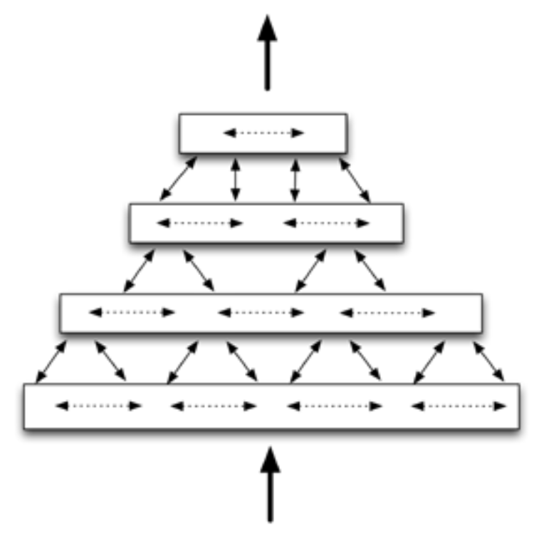
HTM Structure
The HTM network consists of regions arranged hierarchically. Regions are the main components of memory and prediction in HTM, and each HTM region typically represents one level of the hierarchy.
There is always aggregation as you move up the hierarchy. The HTM region is the main building block of memory and prediction in HTM. On the other hand, as we move down the hierarchy, there is divergence of information through feedback connections. (Region and level are almost synonymous. (The term “region” is used to describe the internal function of a region, and the term “level” is used to refer specifically to a region’s role in the hierarchical structure.)

Multiple HTM networks can also be combined. Such a structure is useful when there is data from more than one source or sensor. For example, one network may process audio information while another network processes video information. Each individual network is aggregated toward the top.

The advantage of hierarchical structures is efficiency. It saves a great deal of training time and memory consumption, as patterns learned at each level of the hierarchy can be combined and reused at higher levels. For illustration, consider vision. At the lowest level of the hierarchy, the brain stores information about a small part of vision, such as edges and corners. Edges are the basic building blocks of many objects in the world. These lower-level patterns are aggregated at the intermediate levels into more complex components, such as curves and patterns. An arc could be the rim of an ear, the top of a car handle, or the handle of a coffee cup. These intermediate-level patterns are further aggregated to represent features of higher-level objects such as a head, a car, or a house. When learning a higher-level object, there is no need to relearn its components.
Sharing representations across hierarchical structures also generalizes expected behavior. If we see a new animal, we can predict that it is likely to eat or bite by looking at its mouth and teeth. Hierarchical structures allow us to know that new objects in the world inherit the already known characteristics of their components.
How many things can an HTM hierarchy learn? In other words, how many levels does a hierarchical structure need? There is a tradeoff between the memory allocated to each level and the number of levels needed. Fortunately, HTM automatically learns the optimal representation of each level based on input statistics and the amount of resources allocated. If more memory is allocated to a level, that level will constitute a larger and more complex representation, and thus require fewer levels of hierarchy. If less memory is allocated, it will constitute a smaller, simpler representation and thus require more levels of hierarchy.(See also deep learning techniques.)
region
The representation of regions connected in a hierarchical structure comes from biology. The neocortex is a large skin of neurons 2 mm thick. Biology divides the neocortex into different regions or areas based primarily on how they are connected to each other. Some regions receive input directly from sensors, while others receive input via several other regions. It is the connections from region to region that determine the hierarchical structure.
The details of all the regions in the neocortex appear similar. Despite differences in size and location in the hierarchical structure, the rest of the neocortex is similar. If we slice a 2mm thick neocortical region vertically, we see six layers. Five are cellular layers and one is a non-cellular layer (with a few exceptions, but this is the general rule). Each layer of a neocortical region has many interconnected cells in columns.
HTM regions also consist of a skin of highly interconnected cells arranged in columns. Layer 3 of the neocortex is the main feed-forward layer of neurons. The cells of an HTM region are roughly equivalent to neurons in layer 3 of a neocortical region.

sparse distributed representation
Neocortical neurons are highly interconnected, but are protected by inhibitory neurons so that only a small percentage of neurons are active at any one time. Thus, information in the brain is always represented by a small percentage of the many active neurons. Such encoding is called “sparse distributed representation. Sparse” means that only a small percentage of neurons are active at any one time. Distributed” means that many neurons need to be active to represent something. An active neuron is involved in some semantic representation, but it can only make full sense when interpreted in the context of several neurons.(See also Machine Learning with Sparsity)
HTM regions also use a sparse distributed representation. In fact, the memory mechanism of an HTM region relies on a sparse representation, without which it could not function: its input is always a distributed representation, but it is not necessarily sparse, so the first thing an HTM region must do is convert its input to a sparse representation.
For example, suppose a region receives 20,000 bits of input. The percentage of “1 “s and “0 “s in the input bits will change very frequently over time. The HTM region converts this input into an internal representation of 10,000 bits and stores it within the input. HTM regions convert this input into a 10,000-bit internal representation so that 2% of the input, or 200 bits, are active at any one time, regardless of how many bits of the input are “1’s”. As the HTM region’s input changes over time, the internal representation also changes, but about 200 of the 10,000 bits are always active.
Role of Time
Time plays a pivotal role in learning reasoning. Let’s start with inference. Without time, we can infer almost nothing from tactile or auditory senses. For example, suppose you are blind and someone places an apple on your hand. You can tell what it is by touching it for a few seconds. If you move your finger over the apple, the object itself – the apple and your high-level perception of it – will not change, even though the tactile information is constantly changing. However, if you were told to open your palm and place an apple on it, and you were not allowed to move your hand or fingertips, it would be very difficult to identify it as an apple and not a lemon.
The same is true for hearing. An unchanging sound has little meaning. The word “apple” or the sound of someone biting into an apple can only be understood by a sequence of tens or hundreds of tones that change quickly and sequentially over time.
Sight, by contrast, is a mixed case. Unlike tactile or auditory perception, we can distinguish images even when they pass quickly in front of us for a brief moment. Thus, visual reasoning does not necessarily require temporal changes in input. In normal vision, however, we are constantly moving our eyes, head, and body, and objects are also moving around us. Our ability to make inferences from rapidly changing visual variables is a special case of the statistical properties of vision and years of training. In the general case of vision, hearing, and touch, inference requires temporally varying input.
Now that we have covered the general case of inference and the special case of vision when reasoning about static images, let’s look at learning. To learn, all HTM systems need to be exposed to time-varying input during training. While vision can sometimes reason about static images, to learn what an object looks like, it needs to see the object change. For example, imagine a dog running toward the reader. At each moment in time, the image of the dog forms a series of patterns on the retina in the back of your eye. You perceive these patterns as representing different perspectives of the same dog, but mathematically speaking, they bear little resemblance. The brain knows that these different patterns mean the same thing by observing their sequential changes. Time is the “ancestor” that tells us which spatial patterns appear together.
Note that it is not enough that the input from the sensor changes. A series of unrelated input patterns will only confuse us. Temporally varying input must come from some fixed source in the world. Note also that although we use human sensory organs as examples, non-human sensors are also generally applicable. If we want to train an HTM to recognize patterns of temperature, vibration, and noise in a power plant, the HTM needs to be trained on the data coming from these sensors as they change over time.(See also Time Series Data Analysis)
learning
HTM regions learn about their world by finding patterns and sequences of patterns in the data from sensors. A region does not “know” what its input represents. It only works in a purely statistical world. It sees combinations of input bits that occur frequently and simultaneously. We call these spatial patterns. And it looks at the order in which these spatial patterns appear over time. We call this a temporal pattern or sequence.
If the input to a region is a sensor of the building’s environment, the region will find that certain combinations of temperature and humidity often occur on the north and south sides of the building. They would learn how these combinations change daily.
If the input to a region is information about purchases in a certain store, it will find that certain magazines are purchased on weekends, or that certain price points are preferred in the evening when the weather is cold. It would then learn that different people’s purchase patterns follow similar time series patterns.
An HTM region has limited learning capabilities. A region automatically adjusts what it learns depending on how much memory it has available and how complex the input it receives is. If the memory allocated to a region is reduced, the spatial patterns it learns will be simpler. As the amount of memory allocated to a region increases, the spatial patterns it learns can become more complex. If the learned spatial patterns are simple, a hierarchical structure of regions may be necessary to understand complex images. We can see this feature in the human visual system. Neocortical regions that receive information from the retina learn spatial patterns only for small visual areas. Only after going through several levels of hierarchical structure do they recognize the whole picture of vision.
Like biological systems, the learning algorithms of HTM regions are capable of “on-line learning. Like biological systems, HTM regions’ learning algorithms are capable of “on-line learning,” i.e., they continuously learn as they receive new input. The inference is improved after learning, but there is no need to separate the learning phase from the inference phase. The HTM region also changes incrementally as the pattern of inputs changes.
inference
When an HTM receives input, it matches it with previously learned spatial or temporal patterns. The successful matching of the new input to previously stored sequences is the essence of inference and pattern matching.
Consider how we understand a melody. The first note of a melody is not enough to understand it. If we listen to the next note, the possibilities narrow down considerably, but still not enough. HTM region inference is similar: it looks at the input sequence continuously, but it has not been done before. HTM regions can find matches from the beginning of a sequence, but they are usually more fluid, similar to the way you can understand a melody no matter where it starts. The HTM regions use a distributed representation, so it is more complicated for a region to remember or infer a sequence than in the melody example above. However, this example illustrates how HTM works.
prediction
Each HTM region stores a sequence of patterns. By matching the stored sequence with the current input, we can predict the next input that is likely to arrive. HTM regions actually record transitions between sparse distributed representations. Sometimes the transitions are linear sequences, as in the sounds in a melody, but in the general case many possible future inputs are predicted simultaneously. Much of the HTM memory is used to store sequences and the evolution of spatial patterns.
HTM Implementation
HTM is implemented as nupic and compotex. nupic is implemented in Clojure and htm.core implemented in pyhton. For setting up a Clojure environment, see “Getting started with Clojure” and “Setting up a Clojure development environment with SublimeText4, VS code and LightTable” etc.

コメント