Reinforcement Learning Technology
Reinforcement learning is a type of machine learning that deals with the problem of an agent in an environment observing its current state and deciding what action to take. The agent is rewarded by the environment by choosing an action. Reinforcement learning learns a policy to obtain the most reward through a series of actions. The environment is formulated as a Markov decision process. TD learning and Q learning are known as representative methods.
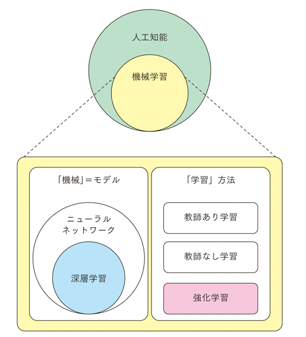
The following is a summary of the relationship between key words surrounding reinforcement learning.

Machine learning is one of the technologies to realize artificial intelligence. Machine learning is literally a method to “learn” a “machine,” and the “machine” is called a model, which in reality is a mathematical formula with parameters. The “machine” is called a model, which is actually a mathematical equation with parameters. “Learning” is the process of adjusting these parameters to match the given data.

Reinforcement learning is different from methods that provide “data” such as supervised data learning and unsupervised data learning, in that it provides an “environment. The environment is defined as a space in which “actions” and changes in “state” in response to actions are defined, and “rewards” are given for reaching a certain state. Simply put, it is like a game. In a game, a character jumps when a button is pressed. Pressing a button” is an action, and “the character jumps” corresponds to a change in state. If the goal is reached, a “reward” is obtained.
In fact, games are a major “environment” used in reinforcement learning, and OpenAI Gym, a library for reinforcement learning in Python, includes games as a reinforcement learning environment.

In the study, the Atari 2600 console game was also used as an environment to measure the performance of reinforcement learning.
In reinforcement learning, the parameters of the model are adjusted so that “rewards” are obtained in the “environment. With Metacar, you can experience how reinforcement learning works in your browser.

Metcar provides a browser-based environment in which the car can be driven and the model can be trained. As a result of learning, it is possible to check which “states” and which “actions” the model values highly.
Reinforcement learning is similar to supervised learning in that there is a “reward” (≒ correct answer) for “action”. The difference from supervised learning is that optimization is performed based on the overall reward (correct answer), not on individual actions. For example, let us consider a case in which a person is given 1000 yen a day, and if he or she endures for 3 days, he or she will be given 10000 yen. There are two actions to be taken: to endure or not to endure.
Since supervised learning evaluates the result of a single action, the optimal action would be the one that does not endure = 1,000 yen. In reinforcement learning, the optimal behavior is to endure for 3 days because the results of the whole and the pupil are evaluated. The period from the start to the end of the environment in reinforcement learning (3 days in this case) is called “one episode,” and the objective of reinforcement learning is to maximize the reward obtained in this one episode.
In other words, in reinforcement learning, “behavior” is evaluated from the viewpoint of whether it leads to the maximization of the “sum of rewards. The model itself needs to learn how to make this evaluation. In other words, a model in reinforcement learning learns two things. The first is how to evaluate actions, and the second is how to select actions (=strategies) based on the evaluation.
Learning how to evaluate actions is the strength of reinforcement learning. In complex games such as Shogi or Chess, it is difficult to evaluate “how good is the current move? However, reinforcement learning learns the evaluation method itself. Therefore, it is possible to learn operations that humans judge intuitively and sensitively.
However, this also means that the evaluation of actions is left to the model. Since people do not give correct answers in the form of labels, it is up to the model to decide what kind of judgment the model will make. This point is also a disadvantage of uninstructed learning. In reinforcement learning, there is a possibility that the model will acquire an evaluation that differs from a person’s senses, resulting in unintended behavior.
When supervised learning is possible, it is preferable to perform supervised learning first. Supervised learning provides labels, so the behavior of the model can be controlled, and it has the straightforward scalability that accuracy simply increases with more data. Reinforcement learning and unsupervised learning each have their merits, but in practice, methods that do not know how they will behave and cannot simply be improved are not welcome.
In this blog, we discuss the following topics.
Implementation
PyTorch is a deep learning library developed by Facebook and provided as open source. It has features such as flexibility, dynamic computation graphs, and GPU acceleration, making it possible to implement a variety of machine learning tasks. Below we describe various examples of implementations using PyTorch.
Reinforcement learning is a field of machine learning in which a learning system called an Agent learns optimal behavior through interaction with its environment. Unlike supervised learning, in which specific input data and output result pairs are provided, reinforcement learning is characterized by the provision of an evaluation signal called a reward signal.
This section provides an overview of reinforcement learning techniques and their various implementations.
Q-Learning (Q-Learning) is a type of reinforcement learning, which is an algorithm for agents to learn optimal behavior while exploring an unknown environment.Q-Learning provides a way for agents to learn an action value function (Q-function) and use this function to select optimal behavior.
The ε-greedy method (ε-greedy) is a simple and effective strategy for dealing with the trade-off between search and exploitation (exploitation and exploitation), such as reinforcement learning. The algorithm is a method to adjust the probability of choosing the optimal action and the probability of choosing a random action.
A Markov Decision Process (MDP) is a mathematical framework in reinforcement learning that is used to model decision-making problems in environments where agents receive rewards associated with states and actions. and Markov properties of the process.
The algorithms integrating Markov decision processes (MDPs) described in “Overview of Markov decision processes (MDPs), algorithms and implementation examples” and reinforcement learning described in “Overview of reinforcement learning techniques and various implementations” are a combined approach of value-based and policy-based methods.
- Algorithms and implementation examples from the integration of inference and action using Bayesian networks
Integration of inference and action using Bayesian networks is a method in which agents use probabilistic models to select the most appropriate action while interacting with the environment, and Bayesian networks are a useful approach for representing dependencies between events and handling uncertainty. In this section, the Partially Observed Markov Decision Process (POMDP) is described as an example of an algorithm based on the integration of inference and action using Bayesian networks.
Thompson Sampling is an algorithm used in probabilistic decision-making problems such as reinforcement learning and multi-armed bandit problems, where the algorithm is used to select the optimal one among multiple alternatives (often called actions or arms) by It is designed to account for uncertainty. It will be particularly useful when the reward for each action is stochastically variable.
The Upper Confidence Bound (UCB) algorithm is an algorithm for optimal selection among different actions (or arms) in the Multi-Armed Bandit Problem (MBA), considering the uncertainty in the value of the actions, The method aims at selecting the optimal action by appropriately adjusting the trade-off between search and use.
SARSA (State-Action-Reward-State-Action) is a kind of control algorithm in reinforcement learning, which is mainly classified as a model-free method like Q learning. After observing the resulting reward \(r\), the agent learns a series of transitions until it selects the next action\(a’\) in a new state\(s’\).
Boltzmann Exploration is a method for balancing search and exploitation in reinforcement learning. Boltzmann Exploration calculates selection probabilities based on action values and uses them to select actions.
A2C (Advantage Actor-Critic) is an algorithm for reinforcement learning, a type of policy gradient method, which aims to improve the efficiency and stability of learning by simultaneously learning the policy (Actor) and value function (Critic).
Vanilla Q-Learning is a type of reinforcement learning, which is one of the algorithms used by agents to learn optimal behavior while interacting with their environment. Q-Learning is based on a mathematical model called the Markov Decision Process (MDP), in which the agent learns the value (Q-value) associated with a combination of State and Action, and selects the optimal action based on that Q-value.
C51, or Categorical DQN, is a deep reinforcement learning algorithm that models the value function as a continuous probability distribution. It has the ability to handle uncertainty by
Policy Gradient Methods are a type of reinforcement learning that focuses on policy optimization. A policy is a probabilistic strategy that defines what action an agent should choose for a state. Policy gradient methods aim to find the optimal strategy for maximizing reward by directly optimizing the policy.
Rainbow (“Rainbow: Combining Improvements in Deep Reinforcement Learning”) is a seminal work in the field of deep reinforcement learning that combines several reinforcement learning improvement techniques into an algorithm that improves the performance of DQN (Deep Q-Network) Rainbow outperformed other algorithms on many reinforcement learning tasks and has become one of the benchmark algorithms in subsequent research.
Prioritized Experience Replay (PER) is a technique for improving Deep Q-Networks (DQN), a type of reinforcement learning. ), and while it is common practice to randomly sample from the experience replay buffer, PER improves on this and becomes a way to preferentially learn important experiences.
Dueling DQN (Dueling Deep Q-Network) is an algorithm based on Q-learning in reinforcement learning and is a kind of value-based reinforcement learning algorithm. Dueling DQN is an architecture for efficiently estimating Q-values by learning state value functions and advantage functions separately, and this architecture was proposed as an advanced version of Deep Q-Network (DQN).
Deep Q-Network (DQN) is a combination of deep learning and Q-Learning, and is a reinforcement learning algorithm for problems with high-dimensional state spaces by approximating the Q-function with a neural network. Learning and uses techniques such as replay buffers and fixed target networks to improve learning stability.
Soft Actor-Critic (SAC) is a type of Reinforcement Learning algorithm that is primarily known as an effective approach for problems with continuous action spaces. Reinforcement Learning) and has several advantages over other algorithms such as Q-learning and Policy Gradients.
Proximal Policy Optimization (PPO) is a type of reinforcement learning algorithm and one of the policy optimization methods, which is based on the policy gradient method and designed for improved stability and high performance.
A3C (Asynchronous Advantage Actor-Critic) is a type of deep reinforcement learning algorithm that uses asynchronous learning to train reinforcement learning agents. A3C is particularly suited to tasks in continuous action spaces and has attracted attention for its ability to make effective use of large-scale computational resources.
Deep Deterministic Policy Gradient (DDPG) is an algorithm that extends the Policy Gradient method (Policy Gradient) in reinforcement learning tasks with continuous state space and continuous action space. deep neural networks to solve reinforcement learning problems in continuous action space.
- Overview of REINFORCE (Monte Carlo Policy Gradient) and Examples of Algorithms and Implementations
REINFORCE (or Monte Carlo Policy Gradient) is a type of reinforcement learning and a policy gradient method. REINFORCE is a method for directly learning policies and finding optimal action selection strategies.
- Actor-Critic Overview, Algorithm, and Implementation Examples
Actor-Critic is an approach to reinforcement learning that combines policy and value functions (value estimators).
- Overview of Trust Region Policy Optimization (TRPO) and Examples of Algorithms and Implementations
Trust Region Policy Optimization (TRPO) is a reinforcement learning algorithm, a type of Policy Gradient, that improves policy stability and convergence by optimizing policies under trust region constraints.
- Overview of Double Q-Learning and Examples of Algorithms and Implementations
Double Q-Learning is a type of Q-Learning described in “Overview of Q-Learning, Algorithms, and Examples of Implementations” and is one of the algorithms of reinforcement learning. It reduces the problem of overestimation and improves learning stability by using two Q functions to estimate Q values. This method has been proposed by Richard S. Sutton et al.
- Overview of Inverse Reinforcement Learning and Examples of Algorithms and Implementations
Inverse Reinforcement Learning (IRL) is a type of reinforcement learning in which the task is to learn the reward function behind the expert’s decisions from the expert’s behavioral data. Usually, in reinforcement learning, a reward function is given and the agent learns the policy that maximizes the reward function. Inverse Reinforcement Learning is the opposite approach, in which the agent analyzes the expert’s behavioral data and aims to learn the reward function corresponding to the expert’s decision making.
- Overview of Maximum Entropy Inverse Reinforcement Learning (MaxEnt IRL) and Examples of Algorithms and Implementations
Maximum Entropy Inverse Reinforcement Learning (MaxEnt IRL) is a method for estimating an agent’s reward function from expert behavior data. Typically, inverse reinforcement learning aims to observe how an expert behaves and find a reward function that can explain that behavior; MaxEnt IRL provides a more flexible and general approach by incorporating the Maximum Entropy principle in the estimation of the reward function. Entropy is a measure of the uncertainty of a probability distribution or prediction, and the maximum entropy principle is the idea of choosing the probability distribution with the highest uncertainty.
- Overview of Optimal Control-based Inverse Reinforcement Learning (OCIRL), Algorithm and Implementation Examples
Optimal Control-based Inverse Reinforcement Learning (OCIRL) is a method that attempts to estimate the reward function behind an agent’s behavior data when the agent performs a specific task. This approach is based on the theory of optimal control theory. This approach assumes that the agent acts based on optimal control theory.
- Overview of ACKTR and Examples of Algorithms and Implementations
ACKTR (Actor-Critic using Kronecker-factored Trust Region) is one of the algorithms of reinforcement learning, based on the idea of the Trust Region Method (Trust Region Policy Optimization, TRPO), It combines Policy Gradient Methods (Policy Gradient Methods) and value function learning, making it particularly suitable for control problems in continuous action spaces.
- Curly Window Search (Curiosity-Driven Exploration) Overview, Algorithm, and Implementation Examples
Curiosity-Driven Exploration is a general idea and method for improving learning efficiency in reinforcement learning by allowing agents to spontaneously find interesting states and events. This approach aims to allow the agent itself to self-generate information and learn based on it, rather than just a simple reward signal.
- Overview of the Value Gradient Method and Examples of Algorithms and Implementations
Value Gradients is a method used in the context of reinforcement learning and optimization that computes gradients based on value functions such as state values and action values, and uses these gradients to optimize measures.
- Active Learning Techniques in Machine Learning
Active learning in machine learning (Active Learning) is a strategic approach to effectively selecting labeled data to improve model performance. Typically, training machine learning models requires large amounts of labeled data, but since labeling is costly and time consuming, active learning increases the efficiency of data collection.
- Overview of Transfer Learning, Algorithms, and Examples of Implementations
Transfer learning, a type of machine learning, is a technique for applying a model or knowledge learned in one task to a different task. Transfer learning is usually useful when a new task requires little data or high performance. This section provides an overview of transfer learning and various algorithms and implementation examples.
The Bandit problem is a type of reinforcement learning problem in which a decision-making agent learns which action to choose in an unknown environment. The goal of this problem is to find a method for selecting the optimal action among multiple actions.
In this section, we provide an overview and implementation of the main algorithms for this bandit problem, including the ε-Greedy method, UCB algorithm, Thompson sampling, softmax selection, substitution rule method, and Exp3 algorithm, as well as examples of their application to online advertising distribution, drug discovery, and stock investment, The paper also describes application examples such as online advertisement distribution, drug discovery, stock investment, and clinical trial optimization, and their implementation procedures.
Simulation involves modeling a real-world system or process and executing it virtually on a computer. Simulations are used in a variety of domains, such as physical phenomena, economic models, traffic flows, and climate patterns, and can be built in steps that include defining the model, setting initial conditions, changing parameters, running the simulation, and analyzing the results. Simulation and machine learning are different approaches, but they can interact in various ways depending on their purpose and role.
This section describes examples of adaptations and various implementations of this combination of simulation and machine learning.
Theory and Application
Reinforcement learning is another aspect of OpenAI, which is famous for chatGPT. The key to GPT is said to lie in the improvement of deep learning models through transformer described in “Overview of Transformer Models, Algorithms, and Examples of Implementations“ based on attention and reinforcement learning as described in “Attention in Deep Learning. When one hears the term “deep learning,” one immediately thinks of its application to games, such as AlphaGo, or to self-driving cars, but this time we will take a more in-depth look at reinforcement learning.
Artificial Intelligence (AI) has great influence in the field of education and has the potential to transform teaching methods and learning processes. Below we discuss several important aspects of AI and education.
- Machine Learning Startup Series “Reinforcement Learning in Python”
- Overview of Reinforcement Learning and Implementation of a Simple MDP Model
An overview of reinforcement learning and an implementation of a simple MDP model in python will be presented.
This section describes the method of planning based on the maze environment described in the previous section. Planning requires learning “value evaluation” and “strategy. To do this, it is first necessary to redefine “value” in a way that is consistent with the actual situation.
Here, we describe an approach using Dynamic Programming. This approach can be used when the transition function and reward function are clear, such as in a maze environment. This method of learning based on the transition function and reward function is called “model-based” learning. The “model” here refers to the environment, and the transition function and reward function that determine the behavior of the environment are the reality.
In this article, we will discuss the model-free method. Model-free is a method in which the agent accumulates experience by moving itself and learns from that experience. Unlike the model-based methods described above, it is assumed that information on the environment, i.e., transition function and reward function, is not known.
There are three points to be considered in utilizing the “experience” of the agent’s actions. (1) accumulation and balance of experience, (2) whether to revise plans based on actual results or forecasts, and (3) whether to use experience for value assessment or strategy update.
In this article, we discuss the trade-off between behavior modification based on actual performance and behavior modification based on prediction. We will discuss the Monte Carlo method for the former and the Temporal Difference Learning (TD) method for the latter. The Multi-step Learning method and the TD(λ) method (TD-Lambda method) are also described as methods that fall between the two.
In this article, I will discuss the difference between using experience for updating “value assessment” or “strategy”. This is the same as the difference between Value-based and Policy-based. We will look at the difference between the two, and also discuss a two-fold approach to updating both.
The major difference between value-based and policy-based learning is the criterion for action selection: value-based learning determines actions to move to the state with the greatest value, while policy-based learning determines actions based on strategy. The former criterion, which does not use strategy, is called Off-policy (no strategy = Off). In contrast, a school building that assumes a strategy is called On-policy.
Take Q-Learning as an example: the target of Q-Learning updates is “value evaluation,” and the criteria for action selection is Off-policy. This is evident from the fact that Q-Learning is implemented in such a way that it “takes action a to maximize value” (max(self.G[n-state])). In contrast, there is a method where the update target is “strategy” and the criterion is “on-policy”. That is SARSA (State-Action-Reward-State-Action).
In this article, we will discuss how to implement value functions and strategies with parameterized functions. This will allow us to deal with continuous states and actions that are difficult to handle in table management.
This time, we describe the implementation by pyhton in the framework of applying deep learning to reinforcement learning.
In this article, I will describe a method of replacing the value evaluation by a function with parameters, which is performed by a table (Q[s][a], Q-table) as described in “Implementation of model-free reinforcement learning in python (1) epsilon-Greedy method” etc. The function to perform value evaluation is called value function. The function that evaluates the value is called a value function, and learning (estimating) the value function is called Value Function Approximation (or simply Function Approximation). In value function-based methods, action selection is based on the output of the value function. In other words, it is a Value-based method.
In this article, we will create an agent that decides its action based on the value function and attack the CartPole environment, which is a popular environment in the OpenAI Gym and is used in various samples. A neural network is used for the value function.
In this article, we describe a game strategy using CNN. The basic mechanism is almost the same as the aforementioned, but the environment is changed in order to experience the advantage of direct screen input. This time, as a specific subject, we will describe Catcher, a game in which vol-catching is performed.
The Deep-Q-Network we have implemented here is currently undergoing many improvements, and Deep Mind, the company that introduced the Deep-Q-Network, has published a model called Rainbow that incorporates six excellent improvements (adding the Deep-Q-Network together makes a total of seven, or seven colors of Rainbow).
A strategy can also be represented by a function with parameters. It is a function that takes a state as an argument and outputs an action or action probability. However, it is not easy to update the parameters of the strategy. In value evaluation, there was a straightforward goal of bringing the estimated value closer to the actual value. However, the action or action probability output from the strategy cannot be directly compared to the value that can be calculated. The expected value of the value would be the learning tip in this case.
Just as we applied DNN to the value function, we can apply DNN to the strategy function. Specifically, it is a function that takes the game screen as input and outputs actions and action probabilities.
There were several variations of Policy Gradient, but here we describe a method called Actor Critic (A2C), which uses Advantage. The name “A2C” itself means only “Advantage Actor Critic,” but the method generally referred to as “A2C” includes methods that collect experience in a distributed environment in parallel. In this section, only the purely “A2C” part is implemented, and the distributed collection is only explained.
A3C (Asynchronous Advantage Actor Critic)” was published before A2C, and it uses the same distributed environment as A2C. The agent not only collects experience in each environment, but also learns. This is “asynchronous” learning (in each environment). However, A “2 “C was created because it was thought that sufficient or higher accuracy could be achieved without asynchronous learning, i.e., two “A “s were sufficient instead of three. Therefore, although it is not Asynchronous learning, the collection of experience in a distributed environment remains.
In “Applying Neural Networks to Reinforcement Learning: Applying Deep Learning to Strategies: Advanced Actor Critic (A2C),” it was mentioned that “Policy Gradient-based methods sometimes have unstable execution results,” and a method to improve this has been proposed. TRPO/PPO, along with the aforementioned A2C/A3C, are currently used as standard algorithms.
In the application of deep learning to reinforcement learning, “value evaluation” and “strategy” were each implemented as a function, and the function was optimized using neural networks. The correlation diagram of the main methods is shown below. There are three negative aspects of reinforcement learning as follows. (1) poor sample efficiency, (2) falling into locally optimal behavior, sometimes overlearning, and (3) poor reproducibility.
In this article, we will discuss methods to overcome the three weaknesses of reinforcement learning: “poor sample efficiency,” “falling into locally optimal behavior, often overlearning,” and “poor reproducibility. In particular, “poor sample efficiency” has become a major issue, and various countermeasures have been proposed. There are various approaches to these problems, but this time we will focus on “improvement of environment recognition.
In “Overview of Weaknesses of Deep Reinforcement Learning and Countermeasures and Two Approaches for Improving Environment Recognition,” I described methods for overcoming three weaknesses of deep reinforcement learning: “poor sample efficiency,” “falling into locally optimal behavior,” “often overlearning,” and “poor reproducibility. In particular, we focused on “improvement of environment recognition” as a countermeasure to the main issue of “poor sample efficiency. In this report, we describe the implementation of these methods.
In this section, we describe research trends in methods other than “improvement of environmental awareness. Specifically, meta-learning and transfer learning are described as “transferability,” intrinsic reward/intrinsic motivation as “improvement of exploratory behavior,” and curriculum learning as “external instruction.
Deep reinforcement learning has the problem of “unstable learning,” which has led to low reproducibility. Not only deep reinforcement learning, but also deep learning generally uses a learning method called the gradient method. Recently, evolutionary strategies (Evolution Startegies) have attracted attention as an alternative learning method to the gradient method. Evolutionary strategies are a classical method proposed at the same time as genetic algorithms and are very simple.
On a desktop PC (64-bit Corei-7 8GM), the above training can be done in less than one hour, which is much shorter than the usual reinforcement learning, and the reward can be obtained without a GPU. Optimization by evolutionary strategy is still under research, but it has the potential to rival the gradient method in the future. Research on the use or combination of other optimization algorithms to improve the reproducibility of reinforcement learning, rather than improving the gradient method, may be developed in the future.
Next, we will discuss how to deal with locally optimal behavior and overlearning. Locally optimal behavior and overlearning are simply “unintended behavior. To solve this problem, “intended behavior” should be learned, and there are two learning methods: “imitation learning” and “reverse reinforcement learning.
In this article, we will discuss various methods of “imitation learning,” in which behavior is evolved from a human model.
Continuing from the previous article, this time we will discuss how to deal with locally optimal behavior and over-learning. Here, we discuss inverse reinforcement learning.
Inversed Reinforcement Learning (IRL) does not imitate the expert’s behavior but estimates the reward function behind the behavior. There are three advantages to estimating the reward function: first, it eliminates the need to design rewards, thereby preventing unintended behavior; second, it can be used for transfer to other tasks, and if the reward function is close, it can be used for learning another task (e.g., learning another game of the same genre); and third, it can be used for human learning. Third, it can be used to understand human (and animal) behavior.
This section describes examples of applications of reinforcement learning and areas where it is expected to be used. Reinforcement learning has been applied mostly to games and automatic driving, but recently, it is being used in areas such as car allocation optimization, and feedback on “how it worked as a result of application” is accumulating, and the cycle of application to the real world is beginning to turn.
Optimization of learning takes advantage of the “reward-based optimization” learning process of reinforcement learning. In recent deep learning models, optimization is often performed by gradient descent, in which case, of course, the “gradient” must be computable. The squared error can be calculated for the gradient, but there are some metrics that cannot be calculated. For example, the gradient of a translation or finally or search system evaluation metric cannot be computed, making it difficult to optimize directly with the gradient method.
With reinforcement learning, even if the gradient cannot be calculated, it can be learned if the value of the evaluation index is set to “reward”. This is the advantage of using reinforcement learning for “learning optimization. In this section, we describe the optimization of the parameters of the model by reinforcement learning and the optimization of the structure.
As examples of optimizing the parameters of a model by reinforcement learning, we describe the creation of a summary and the generation of a chemical structure.
theory
Overview of reinforcement learning techniques. Reinforcement learning is a branch of machine learning that learns sequential decision-making rules. It is the same as operations research in that it aims to optimize decision rules, but it does not assume complete knowledge of the system or environment to which it is applied, but rather the designer inputs “what to do (Goal)” into an algorithm called reward and learns “how to achieve it (How)” from data and other sources. This is a feature of the system.
Therefore, even if you do not have sufficient knowledge of the system, if you can obtain a large amount of data, you may be able to obtain decision-making rules that will achieve your goals through reinforcement learning.
This paper describes the planning problem, which is sequential decision making when the environment is known. The characteristics of the planning problem and the method for solving it provide a basis for dealing with reinforcement learning where the environment is unknown. For example, by studying the characteristics of the planning problem, we can find out which class of measures should be handled even when the environment is unknown. As an established approximation of the planning method, typical methods of reinforcement learning such as the TD method and Q-learning, which will be discussed later, can be derived. In this section, an objective function based on expected returns, optimal value function, and optimal measures are introduced, and a theoretical overview of dynamic programming is given as a method for finding optimal measures.
Continuing from the previous article, I have described the algorithms of the value iteration method and the measure iteration method as specific approaches in dynamic programming for the planning problem of finding optimal measures, assuming that the environment (Markov decision process) is known, without assuming learning from data due to interaction between agents and the environment, etc.
It describes the trade-off between data exploration and utilization, which is a problem in sequential learning of measures from data by collecting data by inputting behaviors and observing rewards and next states in real environments and environmental simulations, and describes a typical measure model that takes the trade-off into account.
In the previous section, we discussed how to decide on a strategy (planning problem) when the environment is known and there is complete information. In this article, we will discuss learning strategies from data obtained through interaction between the agent and the environment, where the environment is unknown. The model-free type of reinforcement learning described here is called environment-de-identified reinforcement learning, which is an approach to learning strategies without explicitly estimating the environment.
Specifically, based on dynamic programming and following the idea of stochastic approximation, we describe a method for performing value iteration from stochastically observed data using the TD method, TD(λ) method, Monte Carlo method, and so on.
Previously, we discussed approximating the Bellman expected operator Bπ from historical data to estimate the value function. In this article, we will mainly discuss learning the optimal strategy π* by approximating the value iteration method based on the Bellman optimal operator B*. However, as mentioned earlier, we cannot simply approximate B* as a sample, so we first define the Bellman action operator and action value function by adding the action space to the Bellman operator and value function. Next, we use them to perform sample approximation of the Bellman action operator. In addition, Q-learning method and SARSA method are described as batch learning and online learning.
In the previous article, we discussed model-free reinforcement learning, in which the environment is not estimated. In this article, we will discuss a model-based type of reinforcement learning in which the environment model is explicitly estimated and the strategy is obtained using the estimated environment model. Specifically, the state transition probability pT and the reward function g of the Markov decision process are estimated from the historical data as the environment model, and the optimal strategy is predicted by using sparse sampling, UCT, Monte Carlo search trees, etc. in the planning method (a method for solving Markov decision processes).
In the case where the number of states is huge or the state space is continuous, it is difficult to learn by approximating the value function and the policy function using a function approximator, because the elements of the table become too large for the conventional table-style function that has a value for each state.
First, we will discuss the case of batch learning, in which the value function is approximated and learned using a function approximator with small degrees of freedom.
In the case where the number of states is huge or the state space is continuous, it is difficult to learn by approximating the value function and the policy function using a function approximator, because the elements of the table become too large for the conventional table-style function that has a value for each state.
First, we discuss the case of online learning (gradient TD learning, least-squares TD learning (LSTD) based on least-squares method, and GTD2 method) in which the value function is approximated and learned using a function approximator with small degrees of freedom. In addition, the choice of function approximations and regularization using LASSO are discussed.
Instead of obtaining measures from the action value function as in the actor-critic method, we consider learning θ by directly specifying a stochastic measure π0 with a measure parameter θ. In this section, we first review the outline of policy learning, and then describe the basics of policy gradient learning, which learns policy parameters according to the gradient method. Finally, we describe an example implementation of the policy gradient method.
When each element of the policy parameter θ corresponds to each state action pair (s,a), θ is practically equivalent to a utility function in table form, which means that we are dealing with a policy model without function approximation. On the other hand, when the number of elements d of the measure parameter θ is smaller than|S||A|, we are approximating the measure with πθ, which is effective when|S| or|A| is large. In particular, when the actions are continuous, the approach of approximating the action value function is often used because it is generally difficult to calculate the action selection and operator argmaxa∈A, etc.
For example, in robot control, a continuous value such as torque becomes an action, and it is desirable to treat the action as continuous rather than simply discretizing it.
Another advantage of directly specifying a strategy by a parameter θ is that the randomness of the action can be automatically adjusted by learning by including such a hyperparameter in the strategy parameter θ, whereas in conventional strategies based on the action value function, the user has to adjust the randomness of the action as a hyperparameter.
Therefore, when it is necessary to find stochastic measures with moderate randomness, it is effective to learn measures by approximating a partially observable Markov decision process (POMDP) as a Markov decision process. It has been shown to be effective in learning strategies by approximating a partially observable Markov decision process (POMDP).
Previously, we assumed that agents can observe states with Markovianity. However, depending on the real problem, the Markovianity assumption may not be realistic, the state may be only partially observable, and future events may depend not only on current observations but also on past history. A mathematical model of such a model is the partially observed Markov decision process.
In a Markov decision process (MDP), the agent (decision maker) can always observe a Markovian state, but in a partially observed Markov decision process (POMDP), the state can only be partially observed, and the process deals with situations where the observed state does not necessarily satisfy Markovianity. In POMDP, the state can only be partially observed, and the process deals with situations where the observed state does not necessarily satisfy Markovianity. For example, when considering the learning of a dialogue agent, the observation is the dialogue partner’s speech, and the action is the agent’s own speech, etc. In many cases, the meaning of the previous speech differs depending on the context of the conversation (speech history), so a Markov decision process cannot adequately model the situation, and a POMDP is used.
As a counterpart to POMDPs, there is another approach for non-Markovian stochastic control processes: predictive state representation (PSR). Broadly speaking, there is a difference between POMDP and PSR in that POMDP represents the state in terms of what was experienced in the past, such as the belief state described below, while PSR represents the state in terms of what is likely to happen in the future.
Assuming that the environmental model P of the POMDP is known, we will explain the planning (finding the optimal measures) method. We have confirmed that the POMDP described above can be attributed to the problem of belief MDPs, but since the belief state is in a continuous space, we cannot use the planning method of a discrete-state Markov decision process directly. Therefore, we show the characteristics of belief MDPs, which are important for deriving planning methods, and describe planning based on dynamic programming. As an implementation example, we describe the exact method and the value iteration method of point approximation, which is an approximate planning method with low computational complexity.
As a planning problem, we deal with the problem of estimating 𝑉∗𝑏. First, we describe the Bellman optimal operator and dynamic programming in belief MDPs, which are the basis for estimating the optimal value function 𝑉∗𝑏.
Finally, as for the implementation, since the summation U of the alpha vectors in the belief space B, which is a continuous space, needs to be computed, it cannot be simply implemented. As an example of an implementation that solves this problem, we describe a rigorous method and an approximate method that reduces the amount of computation and obtains an approximate solution efficiently.
While the application of reinforcement learning is expanding, many cases have been pointed out in which general reinforcement learning methods are difficult to apply. One of the reasons for this is that many reinforcement learning methods aim to maximize the “expected value” of returns. In fact, many cases have been reported that cannot be formulated as problems of maximizing expected returns or minimizing expected costs.
For example, if there is a possibility of a large loss, although the probability of it happening is small, and the user is interested in avoiding the risk as much as possible, the expected return will not be an indicator that correctly reflects the objective. This is because maximizing the expected return reduces the overall cost, but it does not aim to actively avoid the risk of high cost.
In particular, risk aversion is a major theme in financial engineering, and in the case of stock investment, for example, it is necessary to construct a portfolio that increases returns while avoiding large losses that occur with small probability.
Reinforcement learning using deep models is called deep reinforcement learning (DE). In recent years, it has been attracting a lot of attention due to its ability to outperform humans in video games and Go. In this article, we will discuss the topic of deep reinforcement learning.
There are seven methods to improve deep reinforcement learning (original DQN, dual Q-learning (dual DQN method), prioritized experience replay, collision Q-network, distributed reinforcement learning (categorical DQN method), noise network, and n-step cutting return).
I will also discuss alpha-zero, a reinforcement learning method that has been successfully applied to fully informational games such as Go, Shogi, and chess, where only the rules are given and the game is learned from accidental matches to acquire strategies that exceed those of humans.
Temporal difference learning (TD) is one of the reinforcement learning methods and is a value-based method. As shown in equation (1) below, the Q value is determined using an action value function such that the TD error is zero. We explained reinforcement learning here, and here we explain TD learning using a simple Skinner box as an example to understand the implementation of reinforcement learning.
Multi-Task Learning is a machine learning method that simultaneously learns multiple related tasks. Usually, each task has a different data set and objective function, but Multi-Task Learning aims to incorporate these tasks into a model at the same time so that they can complement each other by utilizing their mutual relevance and shared information.
Here, we provide an overview of methods such as shared parameter models, model distillation, transfer learning, and multi-objective optimization for this multitasking, and discuss examples of applications in natural language processing, image recognition, speech recognition, and medical diagnosis, as well as a simple implementation in python.

コメント