Artificial Intelligence Technology Web Technology Knowledge Information Processing Technology Semantic Web Technology Ontology Technology Natural Language Processing Machine learning Ontology Matching Technology
In the previous article, we discussed two methods for calculating similarity: expectation maximization and particle swarm optimization. In this article, we will discuss their extensions to stochastic approaches.
Probabilistic Matching
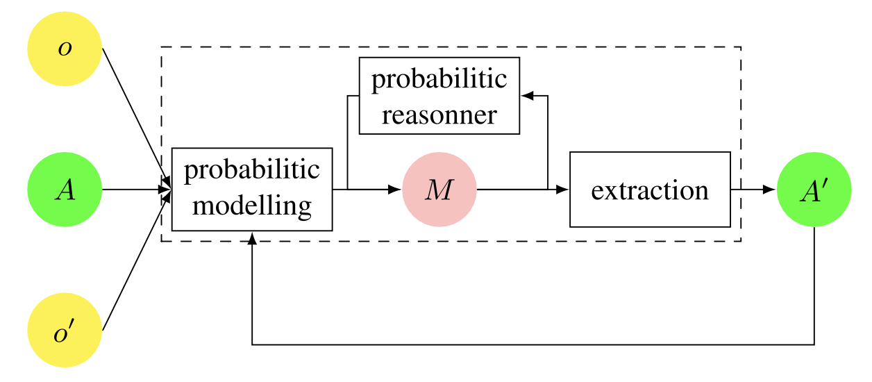
Probabilistic methods are sometimes used universally in ontology matching, for example, to increase the number of available matching candidates. In this section, we introduce several methods based on Bayesian networks, Markov networks, and Markov logic networks. The general framework of probabilistic ontology matching is shown in the figure below.

General setup for probabilistic ontology matching. The matching problem must first be modeled in a particular probabilistic framework, such as a Bayesian network or Markov network. The initialization of the model (network) is performed using a seed match computed on a basic scale or an initial partial alignment between pairs of entities. Probabilistic inference can be performed on the constructed model to compute an enhanced model, which can finally be extracted as an alignment.
Bayesian Networks
A Bayesian belief network or simply a Bayesian network is a probabilistic approach to modeling cause and effect. A Bayesian network consists of (1) a directed acyclic graph containing nodes (also called variables) and arcs (edges), and (2) a set of conditional probability tables. The arcs (edges) between nodes represent conditional dependencies and indicate the direction of influence. For example, an arc (edge) from node X1 (called the parent) to node X2 (called the child) means that X1 has a direct influence on X2. How one node affects another (based on past experience) is defined by the conditional probability table of the node: P (X|parents(X)) is the conditional probability of the variable X, and parents(X) is the set of all and only nodes that directly affect X. The graph and the conditional probability table allow us to find the conditional probability of a variable X. The graph and the conditional probability table give the joint probability distribution of all the variables, i.e.
\[ P(X_1,\dots,X_n)=\displaystyle\prod_iP(X_i|parents(X_i)), \ \ i=1,\dots,n\]
From the above equation, given the value of a node, the probability distribution of the values of other nodes can be inferred. In the simplest case, an expert can specify a Bayesian network, and after some values of the nodes become observable, inferences can be made using them to make predictions and diagnose causes. If not all variables are observable, dependencies between variables need to be specified, which can be solved by learning a Bayesian network that fits the data (Russell and Norvig 1995).
Bayesian networks have been modeled and used in various ways for ontology matching. For example, two ontologies are transformed into two Bayesian networks, and matching is performed as evidence-based inference between these Bayesian networks (Pan et al. 2005). Also, (Mitra et al. 2005) use Bayesian networks to enhance the existing matching by deriving mismatches. The latter will be discussed in more detail.
Bayesian networks, an example taken from (Mitra et al. 2005). Bayesian networks are built with correspondences and use meta-rules based on the semantics of ontology languages that express how each correspondence affects other related correspondences. An external matcher is adapted to generate the initial probability distribution of correspondences, which is then used to infer the probability distribution of other correspondences.

Bayesian network graph. Each node represents a correspondence relationship between ontology entities. The dotted arrows represent the relationships between these entities in the ontology, which induces influence relationships between the correspondences represented by the flat arrows.
Nodes in a Bayesian network graph represent matches between pairs of classes or properties in two different ontologies. The solid arrows in the Bayesian network graph represent the influence between the nodes, while the dotted arrows represent the relations between the target ontologies. For example, the correspondence between the properties hasWritten ∈ o and creates ∈ o′ influences the correspondence between the concepts they have as the ranges Writer ∈ o and Creator ∈ o′ , which in turn influences the correspondence between author ∈ o and hasCreated ∈ o′ . Conditional probability tables are generated using common meta-rules, such as the rule that the probability distribution of a child node is affected by the probability distribution of its parent node. For example, if two concepts Writer and Creator match, and there is a relation hasWritten between Writer and Text in o, and a relation author between Creator and Work in o′, then the probability of match between Text in o and Work in o′ can be The probability distribution of child nodes is constant. The probability distribution of the child nodes is departed from the probability distribution of the parent nodes by using a constant. When the Bayesian network is run, the posterior probability of each node is generated.
Markov Networks and Markov Logic Networks
Next, we will discuss Markov networks (Pearl 1988) and Markov logic networks (Richardson and Domingos 2006). These have been used for ontology matching by (Albagli et al. 2012) and (Niepert et al. 2010), respectively.
A Markov network can be a structured probabilistic network. Similar to Bayesian networks, Markov networks are expressed as N = ⟨V , E⟩ and consist of nodes (V) representing variables and edges (E) between nodes representing statistical dependencies between variables. Specifically, a Markov network represents a joint probability distribution for events represented by variables. Unlike Bayesian networks, Markov networks are undirected. The probability distribution of a Markov network is defined by a potential function (p) for a clique (C), or set of nodes, such that all pairs are connected by at least one edge. A potential or table (pC ) can be associated with each complete subgraph of the network. These correspond to the conditional probabilities of a Bayesian network. The joint distribution of event probabilities as defined in a Markov network is the product of all potentials, i.e.
\[ P(N)=\frac{1}{Z}\displaystyle\prod_{C\in cliques(N)}p_c(C)\]
Z is a normalization constant, also known as the partition function.
Example of a Markov network. Given a pair of ontologies, we need to construct a corresponding Markov network. Similar to the example in Figure 6.6, such a network can be constructed using correspondences, but the solid arrows need to be replaced by undirected edges. A rule to manage the topology of the network could be “if two classes match, then the corresponding parent classes often match as well”. The evidence potential can be initialized by a similarity measure between all pairs of entities, calculated for example through edit distance or user interaction. In the constructed network, probabilistic inference is performed, whereby enhanced alignments are computed. Inference can be done by Monte Carlo methods such as Gibbs sampling or by computing posterior margins, also known as belief propagation. Inference can be done iteratively, or the alignment can be extracted from the network using a threshold of posterior probability.
Markov logic networks (MLNs) are a synthesis of Markov networks and first-order logic. In such a network, nodes represent atomic formulas, and cliques represent the basis of the formulas. As a special case of Markov networks, let us consider a log-linear model. In this case, the potential is replaced by a set of features (formulas) with weights. The probability distribution of the log-linear model is as follows
\[ P(x)=\frac{1}{Z}exp(\displaystyle\sum_i w_if_i(x))\]
Z is a normalization constant, wi is the real-valued weight of feature i, and fi(x) is the i-th feature or first-order logical formula. In this way, a Markov logic network is a weighted first-order logic formula (which determines the graph structure). The grounding of a formula is obtained by replacing all variables in the formula by constants. The higher the evidence that a formula is true, the higher its weight. In this way, the weights indicate how hard or soft the interpretation of the expression is. This makes it possible to deal with uncertainty. That is, in situations where the formula is sometimes violated, it is less likely to be true, but it can still represent a potential correspondence to some extent.
An example of a Markov logic network. Using a Markov logic network for ontology matching, the most probable alignment can be computed given the evidence. The input ontology is assumed to be true knowledge, and is therefore encoded as hard constraints that should hold for all alignments. Initial evidence and weights can be obtained using seed alignments between the entities to be matched. Next, posterior probabilities are calculated for the possible alignments. For example, inference of the maximum posterior probability can be done using integer linear programming. In this formulation of the problem, the objective function to be maximized is: 0.88f1 + 0.1f2 + 0.75f3, where f1 represents the correspondence between entities such as document and document, f2 represents the correspondence between provider and translator, and so on. The weights represent the normative similarity between these entities. These a priori similarities may need to exceed certain thresholds, such as higher than 0.5. integer logic program constraints, such as f1 + f3 ≤ 1, encode cardinality (one-to-one), coherence (avoidance of logical inconsistencies), and structural propagation (in the spirit of Similarity flooding). ). The value of the variable returned by the optimal solution (fi) corresponds to the final similarity.
Summary of Probabilistic Matching
As in many other fields, probabilistic modeling has been incorporated into ontology matching and is being used effectively. However, there are still issues to be addressed, especially in how to obtain a priori probabilities and how to build probabilistic models. For a priori probabilities, it will certainly be more accurate to calculate them based on the task to which the alignment is applied, rather than on syntactic similarity.
However, much more work is needed to better understand the probabilistic basis of ontology matching. In particular, we need to combine probabilistic reasoning with the structure and semantics of alignments and ontologies. This will lead to the more general topic of combining logic and probability, which will also lead to the semantic techniques presented in the next section.
In the next article, I will discuss the semantic approach.

コメント