History of AI and Deep Learning
First, let’s define artificial intelligence (AI). Artificial Intelligence (AI) came into being in the 1950s, when a handful of pioneers in the new field of computer science were pondering whether it was possible to make computers think. The question has yet to be answered, but a simple definition of the field can be summed up as “the effort to automate intellectual tasks that would otherwise be done by humans. This concept encompasses a number of approaches that have nothing to do with learning. For example, early chess programs could not be called machine learning because they only incorporated rules that were hard-coded by programmers.
For quite some time, many experts believed that in order to achieve a level of AI comparable to that of humans, a large number of rules, sufficient to manipulate knowledge, would have to be explicitly defined and manually incorporated by programmers. This idea was the dominant paradigm of AI from the 1950s to the late 1980s. The output of these systems are expert systems.
While the above approaches were particularly suitable for clearly defined logical problems such as a chess match, it was impossible to find explicit rules for solving more complex and fuzzy problems such as image classification, speech recognition, and language translation. Machine learning was born.
The story of machine learning goes back to Victorian England. Countess Ada Laplace was a friend and collaborator of Charles Babbage. Charles Babbage was the inventor of the Analytical Engine, known as the first general-purpose computer. The Analytical Engine was designed in the 1830s and 1840s, and although it was a visionary machine that was well ahead of its time, it was not positioned as a general-purpose computer. This is because the concept of a “general-purpose computer” did not exist at the time.
An analysis engine was merely a means of using mechanical operations to automate certain calculations in the field of mathematical analysis. In 1843, Ada wrote of his invention, “An analytical machine is never a pretentious thing that produces something. It can do anything that it knows how to command to be done. The domain of the analytics community is to help us take what we already understand and make it available.” He stated.
This statement by Ada was later quoted as “Countess Laplace’s Rebuttal” in AI pioneer Alan Turing’s historic 1950 article “Computing Machinery and Intelligence”. In this paper, the Turing test and the main concept of the prototype of AI are proposed. While quoting Ada, Turing discusses whether general-purpose computers can have the ability to learn and be creative, and concludes that they can.
Machine learning stems from the following challenge. Machine learning stems from the following question: “Is it possible for a computer to learn how to perform a specific task on its own, going beyond “what we know how to tell it to do”? This is also a question of whether it is possible for a computer to learn such rules automatically by examining data, rather than manually constructing rules for data processing by a programmer.
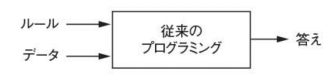
This challenge opens the door to a new programming paradigm. In a conventional program, a person inputs rules (program) and data to be processed according to those rules, and the answer is output. (Figure below)

By introducing the ability to learn into this, when a person inputs data and the answer expected from that data, a rule is output and the rule can be applied to new data to generate a new answer. (Figure below)

Machine learning systems are not explicitly programmed, but rather are trained. Given a large number of samples related to a task, the machine learning system extracts statistical structures from those samples. Eventually, it will be possible to generate rules to automate the task.
For example, let’s say we want to automate the task of tagging photos taken during a vacation. In this case, if you give a sample of pre-tagged photos to the learning system, the machine learning system will learn statistical rules that associate specific photos with specific tags.
Furthermore, if we consider the higher-level intentions of what we want to use the tagged photos for, for example, to create an album, the system will learn rules for selecting tags (photos) that match the layout of the album, or if we want to recreate a specific memory from the past, the system will learn them in chronological order. If you want to recreate a specific memory from the past, you can learn them in chronological order.
Although such machine learning is closely tied to mathematical statistics, there are important differences between the two. Machine learning, such as deep learning, tends to deal with larger and more complex data sets than traditional statistical analysis, such as Bayesian analysis, and as a result, mathematical theory is overshadowed by the emphasis on engineering. Machine learning is a practical field where ideas are experimentally (rather than theoretically) proven.
In order to define deep learning and understand how it differs from other approaches to machine learning, we need to understand “what” machine learning algorithms do. As mentioned earlier, when a sample of what is expected is given to machine learning, it extracts the rules for performing the data processing task. Therefore, in order to run machine learning, we need three things
- Input data points: For example, in a speech recognition task, these data points can be audio files of recorded conversations. For example, in a speech recognition task, these data points could be audio files of recorded conversations. In an image tagging task, these data points could be photos.
- Example of expected output: For example, in a speech recognition task, these data points are audio files of conversations.
- How to evaluate whether the algorithm has done a good job: We need a way to determine the distance between the current output of the algorithm and the expected output. The results will be used as feedback to adjust the way the algorithm works. What we read as “learning” will be this adjustment step.
A machine learning model transforms input data into meaningful output. This becomes a process of “learning” from known samples of input and output. Therefore, the main challenge in machine learning and deep learning is “transforming data in a meaningful way. In other words, machine learning learns useful representations from given input data. These representations are then used to approach the expected output.
Before we move on, let us consider what a representation is. Representation is a way of looking at data from a different angle in order to represent (encode) it. For example, color images can be encoded in RGB (Red-Green-Blue) format or HSV (Hue-Saturation-Value) format. These are two different representations of the same data. For example, the task “select all red pixels in the image” would be easier in RGB format, while the task “reduce the saturation of the image” would be easier in HSV format.
The essence of a machine learning model is to find a suitable representation for the input data (a transformation that makes the data more suitable for the current task, such as a classification task).
As a concrete example, consider the x-axis and y-axis of the xy coordinate system, and the points represented by these coordinates (see below).

In this figure, there are some white points and some black points. Suppose we have developed an algorithm that takes the (x,y) coordinates of a point and outputs the likelihood that the point is black or castle. What is needed here would be a new representation of the data such that white and black points are clearly distinguished. There are various possible transformations, one of which would be a change in coordinates. (Figure below)

In this new coordinate system, we can say that the coordinates of a point are a new representation of data. And it is a good representation. In this representation, the problem of separating black and white can be expressed by the simple rule “black points are points with x>0” and “white points are points with x<0”. With this new representation, the classification problem is essentially solved.
In the above case, the change of coordinates was done manually, but suppose instead that the various coordinate changes are studied in a physical form and the percentage of correctly classified points is used as feedback. In that case, you are piggybacking on machine learning. In machine learning, “learning” represents the process of automatically searching for better representations.
All machine learning algorithms consist of automatically finding such transformations and making the representation more useful for a particular task. They may be transformations of coordinates as described above, or they may be linear projections, or they may be translations (linear projections can destroy information). Or it may be a non-linear operation such as “select all points with x>0”. Machine learning algorithms only search through a set of predefined operations, and usually do not use creativity in searching for such transformations. For this reason, a collection of predefined operations is called a “hypothesis space.
Thus, by technical definition, machine learning is “the search for useful representations of input data in a predefined hypothesis space based on feedback guidance. This simple concept allows for the interpretation of an incredibly wide range of intelligent tasks, from speech recognition to automated driving.
Next, we will discuss the definition of “deep learning”. Deep learning will be a new style of machine learning that learns representations from data. In deep learning, the emphasis is on learning successive layers. The deeper those layers are, the more important the representation becomes. The “deep” in deep learning does not refer to any deeper understanding through this approach. It represents this concept of “successive layers of representation.
The number of layers that make up a data model is called the depth of that model. In this field, it is more appropriate to refer to it as layered representation learning or hierarchical representation learning. In recent deep learning, there are often tens or hundreds of layers of representations. In recent years, deep learning often has dozens or hundreds of layers of representations, all of which are automatically learned from the training data. On the other hand, other approaches to machine learning tend to focus their learning on data representations with one or two layers. For this reason, such approaches are sometimes referred to as shallow learning or surface learning.
In deep learning, these hierarchical representations are (almost always) learned in a model called a neural network. A neural network is really a structure of layers. Although “neural network” is a term from neurobiology, and some of the core concepts of deep learning are developed based on knowledge of the brain, deep learning models are not models of the brain. There is no evidence anywhere that the brain implements the kind of learning mechanisms used in modern deep learning models. Articles in popular science journals claiming that deep learning works like the brain or is modeled after the brain are incorrect.
For those unfamiliar with the field, the idea that deep learning has anything to do with neurobiology is problematic and counterproductive. There is no need to wrap it in a veil of mystery like the human mind. Deep learning is just a mathematical framework for learning representations from data.
The representation that a deep learning algorithm learns is a network consisting of multiple layers, such as the following

The transformation of an image to recognize numbers in an image is done as follows.

This network transforms images of numbers into representations, as shown in the figure above. Those representations gradually change from the original image to different ones, while gradually increasing the information about the final result. As for the deep neural network, it can be thought of as a multi-stage information extraction operation. In this case, the information is gradually “purified” as it passes through the filters one after another, and becomes useful information for some task.
Deep learning can therefore be thought of as a multi-stage method for learning representations of data. These ideas are simple, but scalable enough that they can seem like magic.
As we have seen, machine learning is a mapping from an input, such as an image, to a target value, such as the label “cat”. This mapping is expressed by observing various ensembles of input values and target values. In deep neural networks, the mapping from the input value to the target value is achieved by deeply accumulating simple data transformations (layers), and such data transformations are also learned from samples.
How this learning is done is described below.
The specification of what the layer will do with its input data is stored in the weight of the layer. Basically, weights are represented by a series of numbers. Technically, the transformation implemented by a layer is parameterized by its weights. (see below)

For this reason, these weights are also called parameters of a layer. In this case, learning means finding the values of the weights that correctly map the input values to the customary target values across all layers in the network. The problem here, however, is that a deep neural network can contain tens of millions of parameters. Finding the correct value for each of those parameters can be a daunting task. Moreover, changing the value of one parameter will affect the behavior of all the others.
In order to control something, we must first be able to observe that something. To control the output of a neural network, we must be able to measure how far that output is from what we expect it to be. This is measured by the loss function of the network. The loss function is also called the pbjective function. The loss function supplements the performance of the network in the sample by calculating the loss rate from the predicted value of the network and the true objective value (the value you want the network to output) (see below).

The basic principle of deep learning is to use the loss rate as a backing for the Φ time, and to adjust the weight values little by little. The weights are adjusted in the direction that the loss rate is lower in the current sample.

The weight is adjusted by the optimizer. The optimizer implements an algorithm called backpropagation. Backpropagation is a central algorithm in deep learning, also known as error back propagation.
Since the weights of the network are initialized with random values, it initially simply implements a series of random transformations. Naturally, the output of the network will be far from the ideal output, and the loss will be rather high. However, as the network processes more samples, the weights are adjusted to buy hair in the right direction, and the loss function becomes lower. This is called a training loop, and repeating the training loop a sufficient number of times (usually dozens of times for thousands of samples) produces a value for the weights that minimizes the loss function.
In the next article, I will describe handwritten character recognition by MNIST, which is the Hello World of neural networks.

コメント