R Language Preferences
In this article, I will introduce the actual use of R. First, download R from the official website.
First of all, in order to download R, you need to download the package from the official site according to your OS. Once the installer is downloaded, click on it and follow the instructions to complete the installation.
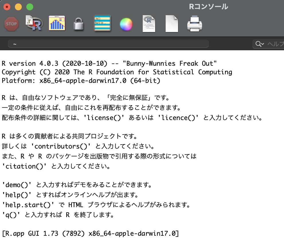
Once the installation is complete, the following screen will appear when you launch the software.

After that, you can enter text next to the “>” as you would in a normal command line tool.
First, create a folder in the desired location to work in (e.g., create a file named R-workspace). Next, change the working directory by typing “setwd(“absolute path of the file”)” in the R console. Next, change the working directory by typing “setwd(“absolute path of the file”)” in the R console. You can check if the change has been made by “getwd()”.
Now let’s try clustering, which is the most common task in practical use. Clustering (cluster analysis) is a data analysis method that divides data into several clusters (groups) based on the similarity of the data, and is called unsupervised learning, where no correct data is given and patterns are found from the input data.
The similarity of data in clustering is based on the distance between the data. The main distances are Euclidean, Minkowski, Manhattan, Mahalanobis, Chebyshev, Canberra, etc. There are many other distances.
There are two clustering methods: k-means, which is non-hierarchical clustering without hierarchy, and hierarchical clustering, which divides the data into several layers. In hierarchical clustering, the distance between the data is judged by a certain rule to form a single cluster, and then the clusters that are close to each other are collected to gradually find a larger cluster. There are several methods for determining the distance between clusters, including the shortest distance method (single linkage method), the longest distance method (complete linkage method), group average method, center of gravity method, median method, McQuitty method, and Ward’s method (minimum variance method).
The data for clustering can be input in CSV format. To load the file, put the data folder in the folder you just created (R-workspace in the example), and set the input data in the following way. (Data created in Excel can also be converted to CSV)
> data <- read.table(“demodata.csv”, sep=”,”, header=TRUE)where data is the variable name, read.table() function reads the data, “demodata.csv” is the name of the data file to be read, sep=”,” is the data separator (“,” since it is CSV here, and header=TRUE specifies whether to read the CSV header. In this case, “demodata.csv” is the name of the data file to be read, “sep=”,” is the data separator (here, “,” since it is CSV, and header=TRUE specifies whether to read the CSV header or not.
This time, we will use the data in R as it is, not from outside. (The dataset we will use is the iris data.) The iris data consists of three types of flowers, 50 samples each, for a total of 150 samples, and four feature values related to the width and length of the sepals and petals. Type “iris” into the console to see the contents of the data. Define the variables and load the data as in the CSV.
> data <- iris[,1:4]
> head(data)
Sepal.Length Sepal.Width Petal.Length Petal.Width
1          5.1         3.5          1.4         0.2
2          4.9         3.0          1.4         0.2
3          4.7         3.2          1.3         0.2
4          4.6         3.1          1.5         0.2
5          5.0         3.6          1.4         0.2
6          5.4         3.9          1.7         0.4
iris[,1:4] indicates that columns 1~4 in the data are to be input, and head(data) is the code to look at the overview of the variable data. Next, let’s look at the structure of the iris data.
> str(iris)
'data.frame':   150 obs. of  5 variables:
 $ Sepal.Length: num  5.1 4.9 4.7 4.6 5 5.4 4.6 5 4.4 4.9 ...
 $ Sepal.Width : num  3.5 3 3.2 3.1 3.6 3.9 3.4 3.4 2.9 3.1 ...
 $ Petal.Length: num  1.4 1.4 1.3 1.5 1.4 1.7 1.4 1.5 1.4 1.5 ...
 $ Petal.Width : num  0.2 0.2 0.2 0.2 0.2 0.4 0.3 0.2 0.2 0.1 ...
 $ Species     : Factor w/ 3 levels "setosa","versicolor",..: 1 1 1 1 1 1 1 1 1 1 ...
If we look at the number of rows of data and the number of data by variety, we see the following
> nrow(iris)
[1] 150
> summary(iris$Species)
    setosa versicolor  virginica
        50         50         50
As for the varieties, we can see that there are 50 samples each for setosa, versicolor, and virginica, for a total of 150 samples.
Now, using clustering, we try to divide the iris into three clusters based on Sepal.Length, Sepal.Width, Petal.Length, and Petal.Width, and classify them by species. Length, and Petal.Width. After clustering, we will check the results against the Species in the dataset to see how accurately we were able to classify the iris by species.
In the next article, we will discuss hierarchical clustering (hclust) and non-hierarchical clustering (kmeans) using this data.

コメント