hierarchical clustering with R
In the previous sections, we discussed the installation of R, the introduction of data, and the preparation of data for clustering, which is frequently used as a practical machine learning application. In this article, we will continue with training and evaluation in hierarchical clustering.
The function hclust for hierarchical clustering is as follows.
hclust(d, method = "使用メソッド")D is the distance, and method is the distance measurement method to be used: single (shortest distance method), complete (longest distance method), average (group average method), centroid (center of gravity method), median (median method), mcquitty (McQuitty method), and ward. D2 (Ward’s method). The execution of the function hclust is as follows.
> distance <- dist(data)
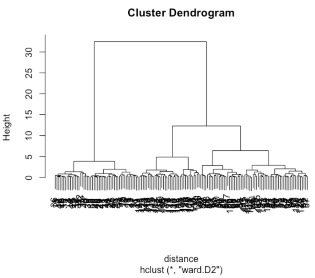
> hc <- hclust(distance, "ward.D2")
> plot(hc)Put the distance obtained by the function dist into the distance variable, and put the value in Ward’s method obtained by the function hclust into the variable hc. Finally, use the plot function to display the result. The result is a dendogram (tree diagram).

To split the data, we use the cutree function, which looks like this
cutree(tree, k = NULL, h = NULL)tree is the data to be split (hc in this case), k is the number of clusters, and h is the height of the tree diagram to be split.。
> result <- cutree(hc,k=3)
> result
[1] 1 1 1 1 1 1 1 1 1 1 1 1 1 1 1 1 1 1 1 1 1 1 1 1 1 1 1 1 1 1 1 1 1 1 1
 [36] 1 1 1 1 1 1 1 1 1 1 1 1 1 1 1 2 2 2 2 2 2 2 2 2 2 2 2 2 2 2 2 2 2 2 2
 [71] 2 2 2 2 2 2 2 3 2 2 2 2 2 2 2 2 2 2 2 2 2 2 2 2 2 2 2 2 2 2 3 2 3 3 3
[106] 3 2 3 3 3 3 3 3 2 2 3 3 3 3 2 3 2 3 2 3 3 2 2 3 3 3 3 3 2 2 3 3 3 2 3
[141] 3 3 2 3 3 3 2 3 3 2
It is confirmed that the data is divided into three categories (1, 2, and 3). Next, substitute the data of the fifth column Species of the iris data into the variable answer, create a cross table of varieties and clustering results, and confirm the classification accuracy.
> answer <- iris[,5]
> table <- table(answer, result)
> table
            result
answer        1  2  3
  setosa     50  0  0
  versicolor  0 49  1
  virginica   0 15 35
From the cross table, we can see that out of 150 samples, (50+49+35=)134 samples were classified correctly.
In the next article, we will discuss k-means, which is a non-hierarchical clustering.

コメント