Statistical Causal Inference and Causal Search
When using machine learning, it is important to consider the difference between “causality” and “correlation”.
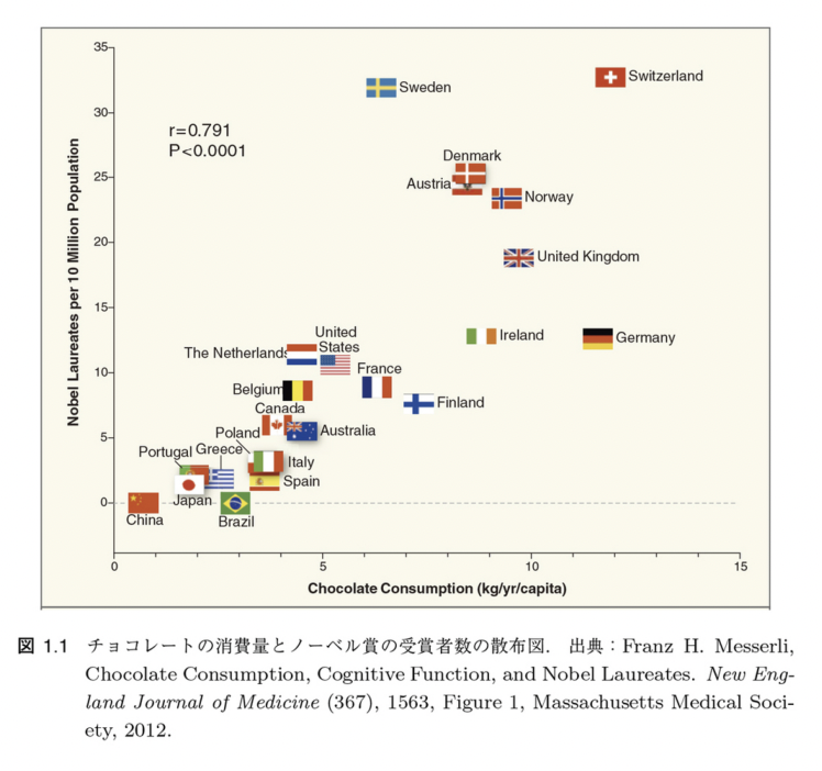
For example, we have the following data on the consumption of chocolate and the number of Nobel Prize winners.

This data clearly shows a correlation between the amount of chocolate consumed and the number of Nobel Prize winners, leading one to conclude that eating chocoholates is the only way to win a Nobel Prize.
In fact, the fact that Switzerland is home to a number of well-known international research institutes, from which a large number of Nobel laureates have emerged, has little to do with the fact that it is the home of chocolate and has a high per capita consumption of chocolate. If you only look at the results of machine learning without considering the original data, you may end up assuming a “causal” or “correlational” relationship with results that happen to be the same as the original data.
To avoid such mistakes, in general natural science experiments, preconditions (experimental conditions) are clearly defined and fixed, and causal relationships are determined by looking at the results when the conditions predicted as causes are changed. In the natural sciences, it is relatively easy to fix preconditions in this way.
On the other hand, in experiments in the humanities (for example, in the social sciences such as the aforementioned chocolate and the Nobel Prize, or in psychology such as people’s reactions when given some kind of trigger), it is difficult to define the factors that affect the results, so methods that randomly vary the possible conditions and then vary the causal A method of varying the parameters is often used. The image is to break the chain of effects by randomizing other conditions.
The techniques to examine such “causal relationships” that are not “correlations” are “causal inference” and “causal search. Both causal inference and causal search are methods for analyzing causal relationships, but there is a difference in purpose and approach: causal inference is a technique for verifying causal relationships, while causal search is a technique for discovering causal relationships.
Causal inference becomes a formal method for identifying causal relationships from experimental or observational data. It would infer that a particular intervention is causing a causal effect by, for example, conducting an experiment on two separate groups and identifying a statistical difference between the two groups. The main approaches to causal inference are (1) “randomized experiments,” in which the intervention variable is randomly assigned to the experiment; (2) “natural experiments,” in which a phenomenon occurring in nature is considered the intervention variable; (3) “propensity score matching,” and (4) “linear regression models,” which statistically estimate causal effects from observed data.
Causal search, on the other hand, is a method for discovering potential causal relationships, which involves searching data to identify variables that may predict outcomes. Specific algorithms include (1) “correlation analysis,” which calculates the correlation between two variables and calculates the correlation coefficient; (2) “causal graph theory,” which creates a directed graph representing the causal relationship between variables and estimates the causal relationship from the graph structure; and (3) “structural equation model,” which constructs a structural equation model representing the causal relationship between variables and interprets the (4) regression analysis, which estimates causal relationships by selecting an appropriate regression model. Various other machine learning algorithms have been applied to causal search.
Various reference books on these causal inferences include “Causal Theory: Reading Causality from Real World Data – Iwanami Data Science 3,” “Statistical Causal Search,” “Causal Analysis with Python: Learning while Making,” “Science of Causal Inference,” “Causality to Understand Philosophy,” “The Identity of Time: Deja Vu, Causal Theory, Quantum Theory,” and others.


These books contain a wide range of information, from philosophical concepts to statistical approaches to various theories and concrete implementations. Various topics picked up from them are discussed below in this blog.
Implementation
Causal inference is a methodology for inferring whether one event or phenomenon is a cause of another event or phenomenon. Causal exploration is the process of analyzing data and searching for potential causal candidates in order to identify causal relationships.
This section discusses various applications of causal inference and causal exploration, as well as a time-lag example.
Causal Forest is a machine learning model for estimating causal effects from observed data, based on Random Forest and extended based on conditions necessary for causal inference. This section provides an overview of the Causal Forest, application examples, and implementations in R and Python.
-
Doubly Robust Learners (Doubly Robust Learners) Overview, Application Examples, and Examples of Python Implementations
Doubly Robust Learners is a statistical method used in the context of causal inference, which aims to obtain more robust results by combining two estimation methods when estimating causal effects from observed data. Here we provide an overview of Doubly Robust Learners, its algorithm, application examples, and a Python implementation.
Concept of causation (philosophical approach)
comming soon
Topics centered on causal reasoning
Causal Inference – Reading Causality from Real-World DataHow to read causality from observational data, especially real-world data that cannot be reproduced. Analysis is difficult due to missing data, bias, and constraints, but this is why there are strong expectations from the field. This book provides an introduction to “causal direction,” “confounding,” and “intervention,” which are essential for scientists and basic education for citizens, as well as analysis methods that are immediately useful.
Various methodologies have been examined for causality as causal inference (statistical causal inference) in data science. First, we will discuss the definitions of correlation and causality.
Correlation is defined as a linear relationship between two variables such that when the value of one variable is large, the value of the other variable is also large (or small).
A causal relationship is said to exist between X and Y when factor Y also changes when factor X changes. Factor X is then called the cause and factor Y is called its result. From here on, variables that indicate causes are called causal variables and variables that indicate results are called outcome variables (outcomes). Manipulating and changing a factor is called intervention or treatment. An intervention can be imagined as providing a treatment or showing an advertisement.
There are many ways to examine causality, adjusting for the effects of confounding factors, but the best way to test causality is through experimental studies. In the field of causal inference, an experimental study is one in which participants are randomly assigned to receive or not receive an intervention, and is called a randomized controlled trial (RCT). In contrast, studies in which the assignment is not random are called observational studies.
In real-life problems, it is unlikely that we know in advance what all the confounding factors are. It is better to assume that there are always unknown confounders. Furthermore, even if a confounding factor is known, it is not always measured, and for a variety of technical and cost reasons, it is not always possible to measure it. In other words, it is best to assume that there are confounders that have not been measured.
Random assignment in experimental studies (RCTs) allows causal inferences to be made without having to worry about any confounding factors, including unmeasured or unknown confounding factors as described above. This is a major advantage of RCTs over causal inference from observational studies. On the other hand, causal inference from observational studies generally requires that confounders be measured. Although some of the methods described below have the potential to address unmeasured or unknown confounders if the conditions are met, the two most basic methods, stratified analysis and regression model analysis, assume that confounders have been measured.
A “correlation” is different from a “causal relationship,” meaning that just because a high correlation is found between one factor X and another factor Y, it does not necessarily mean that there is a causal relationship between them. On the other hand, such a high correlation may be interpreted as a causal relationship. In this issue, we will discuss four typical cases in which “getting caught up in quick correlations can lead to misinterpretation of causal relationships,” and from their causal structures and structural equations, we will discuss the discrepancy between the regression coefficients and the values of the intervention effects.
In this issue, we will discuss the “backdoor criterion”. The backdoor criterion, in a formal description, is indicated by the following two conditions.
Suppose there is a directed path from X to Y in the causal diagram G. Then the following two conditions are satisfied. (1) there is no directed path from X to any element of S, and (2) S is a directed separation of X and Y in the graph from the causal diagram G excluding the arrow line exiting X. The vertex set S satisfies the backdoor criterion for (X,Y).
Another casual definition would be as follows. In the causal structure depicted by the circle and arrow, suppose that there is a path leading to Y when following the arrow downstream from X. In estimating the X→Y intervention effect, a “set of explanatory variables added to the model” that satisfy the following two conditions is said to satisfy the backdoor criterion. (1) The added explanatory variable is not downstream of X. In the causal structure when the arrow exiting from Kyufu X is excluded, the added “set of explanatory variables” blocks all flows affecting both X and Y from common factors upstream (of X and Y).
The backdoor criterion is of broad generality and is important for a unified understanding of the entire field of statistical causal inference.
This section describes how to verify causal relationships for a scenario that is common in the real world, where data comes first and then research queries.
Among the methods for deriving causal relationships from observational data, a relatively robust research method is called a quasi-experiment (Quasi-experiment). While experiments such as randomized controlled trials can prove causality, observational data often fail to show causality. However, a quasi-experiment is a method that demonstrates a causal relationship by creating an experiment-like situation with the observed data. Specific examples of quasi-experimental designs include the following. (1) Instrumental variable design (IV design), (2) Regression discontinuity design (RDD), (3) Interupted time-series analysis), (4) Difference-in-deferrences analysis (DID), (5) Propensity score matching (PS)
- Basics of Statistical Causal Effects (1)Definition of Causal Effects Based on the Rubin Effect Model
In this article, we will discuss the definition and utilization of causal effects based on the Rubin effect model, the most widely used statistical causal effect.
When considering how an action or choice affects the outcome, the counterfactual approach, which compares the current situation with “what would happen if we had done something differently than we actually did,” is quite natural. The Rubin effect model, which is the standard framework for causal effect estimation in statistics, is a statistical framework in which this counterfactual is not just imagined, but is based on data.
Here, we describe the symbols used to explain the Rubin causality model proposed by Professor Rubin of Harvard University in 1970. First, for the sake of simplicity, we assume that there are only two conditions that can be considered as “if…”. The variable Z is a binary variable (Z=1,0), which is an indicator variable for the presence or absence of intervention (or a variable indicating which group a person belongs to), and Y is the value of the outcome variable (outcome). Specifically, Y0 is the outcome variable if the person were subjected to the condition Z=0, and Y1 is the outcome variable if the person were subjected to the condition Z=1.
While causal estimation can be done without considering latent outcome variables by conducting random experiments, there are many cases in which RCTs themselves are difficult to conduct in realistic experiments or could not be estimated by RCTs. In such cases, since all potential outcome variables cannot be observed, some additional assumptions must be made to estimate the ATE. For these cases, we generally make an assumption called “strong ignorability.
If these assumptions hold, we can estimate causal effects using regression models and matching and stratification methods.
The operating variable method has been used in econometrics for a very long time, but it can also be used to estimate causal effects under some conditions, and in relation to the regression analysis design for local treatment effects described below, it has recently become known as the “hidden covariate (i.e., the covariate that cannot be adjusted for by covariate adjustment such as propensity score analysis). It is one of the leading methods for causal effect estimation as “a method that enables bias-free estimation even when confounding factors are present. What does it mean to estimate causal effects using the control variable method? This section describes what it means to estimate causal effects using the operating variable method.
It is often said that “correlation and causation are different,” but the underlying mechanism itself and the extent to which we can distinguish it are two different issues, and what we can do based on limited data and past findings is at best a judgment of “whether there is a high probability of causation.
This time, we describe an example of estimating the causal effect of CM contact (viewing) on app usage as an actual case of causal effect estimation. Specifically, we use single-source panel data in which “TV commercial contact” and “smartphone app use” are obtained from the same subject. The method described here is effective for marketing measures other than TV commercials, and is thought to be useful for implementing the most efficient measures in non-marketing fields where there are residuals and resource constraints.
In the previous section, we discussed the average treatment effect ATE and the average treatment effect ATT in the treatment group as causal effects. ATE is “(average time spent using the application when all people watched the commercial) – (average time spent using the application when all people did not watch the commercial)” in the target population. (average of the current usage time) – (average of the usage time if they were not shown the commercial)”.
In this article, we describe a case in which the theory of covariate adjustment by propensity score is applied to the estimation of the effect of a bunt strategy in baseball. A bunt with no outs is performed with the intention of “sending a runner to second base (scoring position, i.e., if a hit is made, the runner can return to home base) in exchange for a runner on first base with an out count of one. In other words, it is a strategy used to try to score a run. However, even experienced baseball players are divided on whether the bunt strategy really increases the probability of scoring a run. In this article, we will examine whether the bunt strategy is effective (i.e., does it increase the probability of scoring a run?) using data from 2006 to 2014 for games with no outs in the Major League Baseball. (i.e., does it increase the probability of scoring a run?) using data from 2006 to 2014.
One feature of causal inference in the social sciences is the use of non-experimental data. In recent years, field experiments and laboratory experiments have become popular, but most social science research involves the analysis of nonexperimental data because of cost and ethical issues that often prevent experiments from being conducted. The inability to conduct experiments is a major stumbling block to causal inference. However, the development of methods for causal inference under such constraints has been pursued in the field of econometrics, a branch of economics. Here, we focus on “difference-in-differences,” one of the most frequently used methods, and discuss causal inference in the social sciences using nonexperimental data.
Difference in Difference” is called “Difference in Difference” in English and is often abbreviated as DID. Although the basic idea is relatively simple and does not require advanced mathematics, it has a wide range of applications and is a tool that even non-specialists in the social sciences should acquire when considering social issues.
Here, as part of a study aimed at evaluating the effects of childcare leave policies, childcare policies, and other policies on women’s labor, we describe an example of causal estimation on whether the development of licensed childcare centers leads to an increase in maternal employment.
Topics centered on causal search
How do you find cause and effect relationships from huge amounts of data? In this book, the leading researcher who developed LiNGAM (Linear Non-Gaussian Acyclic Model) explains the basics and advanced topics in an easy-to-understand manner. A must-have for causal inference and causal search
The difference between data correlation and causation using the example of chocolate consumption and the number of Nobel laureates. Explains that even though the data appear to be correlated, the number of chocolate consumption and the number of Nobel laureates are not causally related, by testing different causal models assuming unobserved common causes.
The main purpose of substantive science is to clarify causal relationships. The term “substantive science” refers to basic sciences, such as natural and social sciences, and applied chemistry, such as engineering and medicine. Researchers in real science have a specific phenomenon they want to elucidate or problem they want to solve. For example, “Will taking this medicine cure that disease?”, “Will increasing sleep hours reduce depressive mood?
In contrast to substantive science, statistics and machine learning are called mrthodology. Methodology researchers study the methods themselves to achieve the goals of real science. For example, researchers in statistics and machine learning create or elaborate data analysis methods.
Statistical causal inference becomes a methodology for inferring from data about causal relationships. Roughly speaking, if you change something and something else changes, the two are causally related. So, how can we mathematically express that when we change something, something else changes (or does not change)?
In this article, I will discuss the counterfactual model, which is a concept of causality adopted in statistical causal inference, and a mathematical model called the structural equation model, which is a tool for describing the process of data generation, and based on these two, I will discuss the structural causal model, which is a mathematical framework for causal inference.
In the previous article, we discussed the definition of causality by the counterfactual model and the structural equation model. In this article, I will discuss structural causal models and randomized experiments.
The structural casusal model, which is a typical framework for causal inference, is based on two models. One is the counterfactual model, which is a model of causation, and the other is the structural equation model, which is a model of the data generation process. In this section, the causal relationships defined in the counterfactual model are mathematically expressed using the structural equation model.
First, we will express the causality at the population level in the counterfactual model using the structural equation model. First, an action called “intervention” is defined using a structural equation model. To intervene in a variable x means to “take the value of variable x to be a constant c, no matter what value any other variable takes. The other variables are all variables, both observed and unobserved. This kind of intervention is denoted by the symbol do, do(x=c). Incidentally, where the intervention comes from is from outside the model. It is up to the analyst to decide which variables to include in the model. In other words, it is the analyst who decides what is inside and outside the model.
The study of statistical causal inference can be divided into two main categories. The first is to determine under what conditions predictions and explanations about causality can be made, assuming that the causal graph is known. The other is to clarify under what conditions causal graphs can be inferred, assuming that they are unknown. The point of view that divides the two is whether the causal graph is known or unknown. The approach in which the causal graph is unknown is called statistical causal search.
There are three main approaches to the basic problem of causal search. The first is the non-parametric approach, in which no assumptions are made on the functional form or the distribution of the exogenous variables. The second is the parametric approach, which incorporates the prior knowledge of the analyst into the model as a process and makes assumptions on both the functional form and the distribution of the exogenous variables; the third is the semi-parametric approach, which makes assumptions on the functional form but not on the distribution of the exogenous variables.
Three approaches, nonparametric, parametric, and semiparametric approaches, are compared in terms of identifiability of causal graphs. A causal graph is said to be identifiable if “the distribution of function approximations is different if the structure of the causal graph is different” under a certain assumption. On the other hand, if “the distribution of function approximations can be the same even if the structure of the causal graph is different,” then the causal graph is not identifiable.
Here, the constraints are too loose to result in an unclear model, so we add constraints. A typical assumption to add is: “The error variables ei(i=1,…,p) are independent. ,p) are independent. This assumption implies that there is no unobserved common cause. The next most common assumption is that causality is acyclic.
This section compares the nonparametric, parametric, and semiparametric approaches to statistical causal search.
First, we summarize the characteristics of the nonparametric approach. One of the standard principles for inferring causal graphs is the causal Markov condition, which is an inference principle based on the conditional independence between observed variables. The causal Markov condition states that each variable is independent of its non-descendant variables when conditioned on its parent variables.
This condition holds in general for acyclic structural equation models without unobserved common causes (i.e., the causal graph is a directed acyclic graph), not only in the linear case as in equation (5), but also in the nonlinear and discrete variable cases. Therefore, in the nonparametric approach, where no assumptions are made on the functional form or the distribution of error variables, causal Markov conditions are used to infer the causal graph.
In order to infer the causal graph, the causal Markov condition alone is not sufficient; an additional assumption called faithfulness is required.
In the framework of the nonparametric approach, we will discuss approaches for inferring causal graphs from actual data. There are two major inference approaches.
The first is called the constrained-based approach. In this approach, we first infer from the data what independence is possible for the function approximation. The next step is to search for a causal graph that satisfies the inferred conditional independence as a constraint. A typical estimation algorithm is the PC algorithm (Peter and Clark, PC algorithm).
The other is called the score-based approach, which evaluates the goodness of the model for each Markov equivalence, which is a set of causal graphs that give the same conditional independence.
I will discuss the LiNGAM model, which is a typical model of semi-parametric approach in the case of no unobserved common cause, in which the causal graph can be uniquely inferred using the non-Gaussian nature of the distribution of observed variables.
In this article, we will discuss a structural causal model called the LiNGAM model (linear non-Gaussian acyclic model). For this purpose, we first describe a signal processing technique called independent component analysis.
Independent component analysis (ICA) is a data analysis method that has been developed in the field of signal processing. Independent component analysis considers that the values of observed variables are generated by mixing the values of unobserved variables. For example, the voices of multiple speakers are mixed together and observed by multiple microphones.
Among the semiparametric approaches, we describe the LiNGAM model, a model in which the causal graph is identifiable.
The approach is based on the aforementioned independent component analysis, and the inference of the coefficient matrix in the structural equation model is performed by obtaining a transformation matrix that rearranges the causal order so that the diagonal components of the restoration matrix related to the coefficient matrix are not zero.
The estimation method of the coefficient matrix B of the LiNGAM model is described in detail. There are two main approaches. One is to employ the method of independent component analysis, and the other is to repeat the regression analysis and independence evaluation. Both estimation approaches estimate the coefficient matrix B in two steps. In the first stage, the causal order K(i)(i=1,…. p) of the observed variables xi is estimated. As mentioned above, the causal order K(i)(i=1,…,p) of the observed variables xi is estimated. .p), the coefficient matrix B becomes a strict lower triangular matrix. Therefore, all components of the upper triangle of the coefficient matrix can be estimated to be zero. In the second stage, we estimate the remaining lower triangular components.
In this article, we describe the specific approach using independent component analysis (Hungarian method) and regression analysis (adaptive Lasso)
For an approach to estimate the causal order of observed variables xi one by one, starting from the earliest one, by repeating regression analysis and examination of independence.
To consider the LiNGAM model and its estimator in the presence of unobserved common causes, we begin with an example of using data to infer causality: suppose we are interested in the causal relationship between two observed variables x1 and x2. We assume acyclicity and consider estimating the direction of causality between the two variables and the magnitude of the causal effect. We compare the three models using the framework of a structural causality model to represent such causality.
The independent component analysis approach would explicitly incorporate unobserved common causes into the model. In this case, the number of unobserved common causes must be identified, but it is natural to assume that they are generally innumerable, and it is often difficult to estimate the appropriate number from the data.
An approach that does not explicitly incorporate unobserved common causes into the model is to introduce a sum of unobserved common causes, which does not introduce unobserved common cause variables.
The characteristic feature of this mixed model-based approach is that unobserved common causes are not entered into the model individually, but rather as a sum. Thanks to this, there is no need to model the distribution of unobserved common causes individually, nor to estimate their number or coefficients. Instead, we need to include the intercept of each observation as a parameter in the model. Since each of the variables x1 and x2 has its own intercept, we need an intercept parameter twice as large as the lower figure of observations.
Research has been conducted to determine how far the assumptions of the LiNGAM approach of linearity, acyclicity, and non-Gaussianity can be loosened. Here, we describe a representative extension of the model.
Currently, most of the studies are for the case of no unobserved common cause, but based on these studies, we are gradually moving toward the case of unobserved common cause. If we do not do something about unobserved chest pain causes, the fundamental issue of causal search, the problem of pseudo-correlation, will remain
The question of whether there is a causal relationship from one time series to another assumes that at least two time series data are of interest. Causal inference based on time series is essentially a multivariate time series problem, and multivariate autoregression models (Vector AutoRegression model, VAR model) are often used as models.
Here, we describe the procedure for analyzing causality based on the VAR model, using the free software R as an example of the causal relationship between the approval rating of the Cabinet and stock prices. Data often contain missing data, and the Cabinet approval rating, which is the subject of this paper, is no exception. In this section, we will discuss interpolation of deficient values using the function decomp included in the timsac package of R. In addition, since causal analysis using the VAR model assumes stationarity of time series, it is necessary to check for stationarity and non-stationarity and to perform preprocessing to make the time series stationary. The procedure for this and the use of the unit root test are also described. The R package vars is used for estimation of uncontrolled/controlled VAR models, lag selection, causality tests, and calculation of impulse response functions.
In this section, we introduce the multivariate autoregressive model (VAR model) as a framework for analyzing the causality of time series. vars. A time series xt to yt is said to be “causal in the Granger sense” when the past values of other time series xt are useful in predicting time series yt.

コメント