Principle Component Analysis (PCA)
In the section on the beginning of modern deep learning technology, autoencoders, I mentioned that the paper by Hinton et al. gave PCA as a precedent. In this article, we will discuss PCA in more detail.
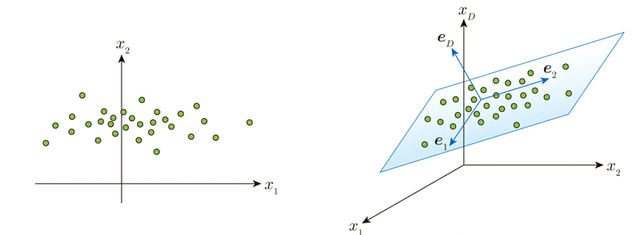
PCA is a method of dimensionally compressing multidimensional data, for example, assuming data in a two- or three-dimensional space, and as shown below, if the data is uneven (large variance) on a specific one-dimensional axis (straight line) or two-dimensional axis (plane), the data is assumed to be unbalanced on that straight line or plane, and the original two-dimensional or three-dimensional axis is used instead. When the data is uneven (high variance) on a straight line or plane, it is represented as data on a specific 1D axis (straight line) or 2D axis (plane) instead of the original 2D or 3D axis.

機械学習プロフェッショナルシリーズ「これならわかる深層学習入門」より*1)
The actual algorithm assumes a basis vector e that represents a new subspace (a specific 1D axis or 2D axis as described above), and calculates the minimum or problem min E(c0, e) using the median (mean) of the data distribution c0, using the Lagrangean undecided coefficient method. For more information on the Lagrange multiplier method, see “Dual Problem and Lagrange Multiplier Method.
Let’s try to perform a principal component analysis using R. The reference is from “The Concept of Principal Component Analysis” by Shinya Baba.
First, we use the iris data that R comes with by default, and draw a graph using the two packages “ggplot2” and “GGally”.
install.pacjages("ggplot2")
install.packages("GGally")
library(ggplot2)
library(GGally)
ggpairs(iris, aes_string(color="Species", alpha=0.5))
Use the drawing function “ggpairs” with the argument “sea_string(color=”Specis”, alpha=0.5)” to add color to each type. alpha=0.5 specifies the transparency. The result is as follows.

The results are displayed for each variable. The scatter plot shows the distribution of each variable as xy, the correlation coefficient for the data in the target position to the scatter plot, the smoothed histogram for the variable if the vertical and horizontal are the same, and the last column is a box-and-whisker diagram by type.
We now perform a principal component analysis (using the “procomp” function).
#種類データを除く(procompでは種類のデータに適用できない為)
pca_data <- iris[,-5]

#主成分分析の実行
model_pca_iris <- procomp(cpa_data, scale=T)

> # 結果
> summary(model_pca_iris)
Importance of components:
                        PC1     PC2    PC3     PC4
Standard deviation     1.7084 0.9560 0.38309 0.14393
Proportion of Variance 0.7296 0.2285 0.03669 0.00518
Cumulative Proportion  0.7296 0.9581 0.99482 1.00000

# 主成分分析の結果をグラフに描く
install.packages("devtools")
devtools::install_github("vqv/ggbiplot")
library(ggbiplot)

ggbiplot(
  model_pca_iris,
  obs.scale = 1,
  var.scale = 1,
  groups = iris$Species,
  ellipse = TRUE,
  circle = TRUE,
  alpha=0.5 )
The results are as follows.

iris pca結果
It is confirmed that Petal.Length and Petal.Width have almost the same axis. Length is also quite close in direction. On the other hand, Sepal.Width clearly has an axis in a different direction. From the above, we can conclude that Petal.Length, Petal.Width and Sepal.Length are the first principal component axes and Sepal.Width is the second principal component axis. Length and Sepal. Width are the first and second principal component axes, respectively. In fact, looking at the distribution of the iris data above, the histogram distribution of Sepal.
As a development of PCA, there are correspondence analysis (applicable to categorical data, etc.), kernel principal component analysis (applicable to nonlinear data), principal component regression (using the results of principal component analysis to perform regression analysis and make predictions), etc.
References *1) This is a good introduction to deep learning.
Robust Principal Component Analysis, which is also described in “Overview of Robust Principal Component Analysis and Implementation Examples” is a method for finding a basis in data and is characterized by robust operation even with data that contains outliers and noise.

コメント