Summary
From “Using Algorithms in Problem Solving and Training Coding Techniques“. I will discuss some basic algorithms for graph data (DFS, BFS, bipartite graph decision, shortest path problem, and minimum global tree).
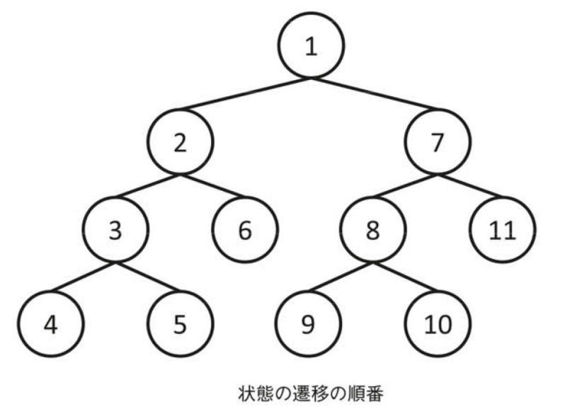
depth first search (search algorithm in AI)
First, let’s talk about Depth-First Search (DFS), which is a search method. DFS is a search method that starts from a certain state, advances through the states until the transition is no longer possible, and then returns to the previous state when the transition is no longer possible. For example, in the case of sudoku, you start with an appropriate square, determine the value of another square, and so on, until you reach a solution. Depth-first search can often be solved easily using the recurrence function due to its nature.

Here, a recursive function refers to calling the same function within a function. For example, if you want to create a function int fact(int n) that calculates factorial, you can write it as follows since n!=nx(n-1).
int fact(int n) {
  if (n == 0) return 1;
  return n * fact(n-1);
}
Whenever you write a recursive function, you need to make sure that the function stops. In the previous example, when n=0, the function returns 1 directly instead of calling fact again. Without this condition, the function will be called infinitely and the program will run out of control.

Depth-first search generates all the states that can be reached by rearranging the transitions from the first state. Therefore, it is possible to perform operations on all states and to enumerate all states.
In depth-first search, a stack is basically used. The stack is a data structure that can perform two operations: push and pop. Push is an operation to pile data on top of the stack, while pop is an operation to remove data from the top of the stack. In other words, the last element is taken out first, so it is called LIFO (Last in First Out).

Stacks can be easily created using arrays or lists, but they are provided as standard in most programming languages and can be used. Also, since function calls are usually realized on the stack, the recursive functions described above can be rewritten using the stack instead of recursive calls.
breadth-first search
Next, we will discuss breadth-first search (BFS: Breath-Fisrt Search), which is another basic search method that, like depth-first search, searches for all states that can be reached from a given state for the first time.
The difference between BFS and depth-first search is the order in which the states are searched, i.e., in breadth-first search, the states are searched from the one closest to the first state. In other words. In other words, the order of search is as follows: initial state -> all states that can be reached in the shortest one transition -> all states that can be reached in the shortest two transitions -> —. In breadth-first search, the same state is passed through only once, so the computational complexity is about O(number of states x number of transitions).

While depth-first search uses a stack, breadth-first search uses a queue. First, the initial state is put into the queue, then the state is taken out of the queue and put into the queue of all unvisited states that can be transitioned from there, and the operation is repeated until the queue is empty or a turn is found. If you look at the queue, you can see that the states are coming out in the order of their initial state.
Here, the Queue is a data structure that can perform two operations, push and pop, just like the stack. What is different from the stack is that pop is not retrieved from the top, but from the bottom. In other words, the element that is placed first comes out first. This is called FIFO (First in First Out).

In width-first search, the search is done in the order of closest to the initial state, so it is easy to find the shortest path, shortest number of moves, etc. If the state is simple, for example, just the coordinates of the current position, the state can be represented by creating a pair or encoding it as an init type. If the state is more complex, it is necessary to create a class to represent the state. Transitions can be made in four directions for planar movement, but it is necessary to consider the dimensions depending on the problem.
In a breadth-first search, if we only keep a graph that indicates whether we have already visited a place, we can search from the closest one. In the case of a problem that requires the shortest distance, we define an array that stores the shortest distance, and initialize the array with a sufficiently large constant INF, for example, so that the places that have not yet been reached become INFs and can play the role of flags at the same time.
The search is terminated when the goal is reached, but if the search is not terminated and continues until the queue is empty, the shortest distance to each point can be calculated. If the shortest distance array is INF after searching until the end, it means that the starting point is unreachable.
Width-first search, like depth-first search, generates all the states that can be reached. Therefore, we can use breadth-first search when we want to process all the states. However, recursive functions are often drawn in depth-first search because they are shorter and it is easier to store the states. On the other hand, if you want to find the shortest path, BFS is used because DFS will take you through the same state many times.
The following is a description of the basic tree structure data algorithm using them.
two-part graph decision
First, let’s talk about the “n-partite graph decision. In this algorithm, given an undirected graph with n vertices, we color the vertices so that adjacent vertices are colored differently from each other, and determine whether all vertices can be colored within two colors.
The problem of coloring adjacent vertices so that they are colored differently from each other is called a graph coloring problem. The minimum number of colors required to color a graph is called the graph coloring number. A graph with a coloring number of 2 is called a bipartite graph. A bipartite graph is an important graph structure that can be used as a base when learning relational data.

In the case of painting with two colors, once the color of one vertex is determined, the colors of the adjacent vertices are also determined uniformly. Therefore, by starting from an appropriate vertex and sequentially deciding the colors of the neighboring vertices, we can determine whether two colors are wet or not. This can be easily written by using depth-first search.
If. If the graph is connected, we can look at all vertices in a single DFS. DFS can also be used to find the topological order.
Next, we will discuss the shortest path problem. The shortest path problem is one of the most fundamental problems in graphs. Given two vertices, the shortest path is the one that minimizes the cost of the edge through the path that starts and ends at the vertices. It is easy to understand the shortest path by considering the cost as the distance.

Bellman-Ford law
First, let’s talk about the Bellman-Ford method. When the starting point is fixed, the problem of finding the shortest distance between all other vertices is called the single starting point shortest distance problem. Furthermore, the one with a fixed endpoint is called the grandfather vertex-to-shortest path problem, but it is solved by the single starting point shortest path problem since it can be solved with the same amount of computation.
Let d[i] be the shortest distance from the starting point s to the vertex i. Then we have the following equality.
\[d[i]=min\{d[j]+(Cost\ of\ an\ edge\ from\ j\ to\ i)|e=(i,j)\in E\}\]
If the graph is a DAG, then the vertices can be ordered and d can be calculated using this asymptotic formula. However, if the graph contains closed paths, it is not possible to order them. If this is the case, and if the tentative shortest distance is d[i], and the initial values d[s]=0 and d[i]=INF (a sufficiently large constant), then d can be calculated by repeatedly applying this formula and updating d. If there is no closed circuit, this update will stop sometime, and d at that time will be the shortest distance.
//Edge with cost cost from vertex from to vertex to
struct edge { int from, to, cost;};

edge es{max_E];  //edge

int d[MAX_V];   //shortest distance (to)
int V, E;       //V is the number of vertices, E is the number of edges

// Find the shortest distance from the sth vertex to each vertex.
void shortest_path(int s) {
  for (int i = 0; i < V; i++) d[i] = INF;
  d[s] = 0;
  while (true) {
     bool update = false;
     for (int i = 0; i < E; i++) {
        edge e = es[i];
        if (d[e.from] !=INF && d[e.to] > d[e.from] +e.cost) {
          d[e.to] = d[e.from] + e.cost;
          ipdate = true;
        }
      }
      if (!opdate) break;
    }
 }
This algorithm is called the Bellman-Ford method. If the graph does not have a closed path with negative cost reachable from s, the shortest path will not pass through the same vertex, so it will be executed only at most|V|-1 times. This algorithm can also be used to detect all fucyrons by initializing d[i]=0 for all i.
Next, we will discuss the Dijkstra method. If there are no negative edges and d[i] is not the shortest distance by the Bellman-Ford method, d[j] will not be the final shortest distance even if it can be updated to d[j]=d[i]+(the cost of the edge from i to j). Also, even if d[i] does not change, we are still looking at the edge coming out of vertex i each time, which is useless. So we modify it as follows.
- Update the vertices that are adjacent to the vertex whose minimum distance has been determined.
- We no longer use the vertex with a fixed shortest distance that we used in step 1.
Dijkstra method
The question is how to find the vertex with the fixed shortest distance among 1 and 2. In the initial state, only the starting point has a fixed shortest distance. Of the vertices that have not yet been grabbed, the vertex with the smallest distance d[i] has a fixed shortest distance. This is because there are no negative edges, so the distance cannot become smaller after d[i]. This algorithm is called Dikstra’s method.

int cost[MAX_V][MAX_V];  //cost[u][v] is the cost of the edge e(u,v) (or INF if it does not exist)
int d[MAX_V];            //Shortest distance from vertex s
bool used[MAX_V].        //Flag already used
int V;

//Find the shortest distance from the starting point a to the extended point.
void dijkstra(int s) {
   fill(d, d + v, INF);
   fill(used, used + V, false);
   d[s] = 0;

   while(true) {
     int v = -1;
     //Find the vertex that has not yet been used and has the smallest distance.
     for (int u = 0; u < V; u++) {
       if(!used[u] && (v == -1 || d[u] < d[v])) v = u;
     }
     if (v == -1) break;
     used[v] = ture;

    for (int u = 0; u < V; u++) {
      d[u] = min(d[u], d[v] +cost[v][u]);
    }
   }
 }
Walsall-Floyd process
Finally, we discuss the Worshall-Floyd method. The problem of finding the shortest path between all two vertices is called the all points-to-shortest path problem. The all-point-pair shortest path is obtained by DP. Let d[k+1][i][j] denote the shortest path from i to j when only vertices 0 to k and i, j are used, and d[0][i][j]=cost[i][j] when k=-1, assuming only i and j are used. The case where only vertices 0 to k are used is attributed to the case where only vertices 0 to k-1 are used.
When using only vertices 0 to k, the shortest path from i to j can pass through vertex k exactly once or not at all. If it does not pass through vertex k, then d[k][i][j]=d[k-1][i][j]. If it passes through vertex k, it decomposes into the shortest path from vertex i to vertex k and the shortest path from vertex k to vertex j, so d[k][i][j]=d[k-1][i][j]+d[k-1][k]i. Putting these two together, we get d[k][i][j]=min(d[k-1][i][j],d[k-1][i]k]+d[k-1][k][i]). This DP will use the same array and update it as d[i][j]=min(d[i][j],d[i][k]+d[k][i]).
This algorithm is called the Warshall-Floyd method, and it can find all points versus the shortest path in O(|V|3). Like the Bellman-Ford method, the Warshall-Floyd method also works even if there are negative edges. Whether or not there is a negative closed path can be determined by whether or not there is a vertex i for which d[i][i] is negative.
int d[MAX_V][MAX_V]; //d[u][v] is the cost of edge e=(u,v) (or INF if it does not exist, but d[i][i]=0)
int V; //Number of vertices

void warshall_floyd() {
  for (int k = 0; k < V; k++)
     for (int i = 0; i < V; i++)
        for (int j = 0; j < V; j++) d[i][j] = min[d[i][j], d[i][k] + d[k][j]);
}
All the point-to-point shortest paths can be found in a very simple triple loop. Since it is easy to implement, the Worchal-Freud method should be used even for the single starting point shortest path problem, if there is room for computation.
minimum-width tree algorithm
Next, I will describe the algorithm for the minimum total area tree. Given an undirected graph, a spanning tree is a subgraph of the undirected graph such that any two vertices are connected. If an edge has a cost, a spanning tree that minimizes the sum of the costs of the edges used is called a minimum spanning tree (MST).
For example, consider a graph where the vertices are villages and the edges are roads to be built. A minimum spanning tree is equivalent to building exactly one road for every village, so that every village can be reached. If the road has a construction cost, the minimum whole area tree problem can be thought of as making the whole area tree so that it has the minimum construction cost.

Algorithms for finding the minimum global tree are known as Kruskal and Prim methods. Obviously, the existence of a global tree is equivalent to its being connected, so we assume that the graph is connected.
PRIM method
First, let us discuss the minimum global tree problem using the Prim method. The prim method is similar to the Dijkstra method, starting from a vertex and gradually adding edges.
First, consider a tree T with only one vertex v. From here, we greedily add edges of minimum cost connecting T with other vertices to T repeatedly to construct the whole tree. We will prove that the global tree constructed in this way is a minimum global tree.

Let V be a set of vertices. Suppose that we now have a global tree T for X(⊂ V), and that there exists a minimal global tree such that T is a subgraph of T. We show that there exists a minimal global tree of V that contains an edge of minimal cost connecting X and VX and that has ka as a subgraph. Let e be a minimum cost edge, and let v(∈ X) and na ∈ VX) be connected. There exists a minimal global tree of V such that it contains T as a subgraph by assumption. e is not contained in this minimal global tree, since there is nothing to say if e is contained in it. Since the global tree is a tree, we can create a closed path by adding e.
Among the edges in the closed path, there is always an edge f that connects X and VX and is different from e. The cost of f is more than the cost of e because of the way e is scattered. Therefore, by removing f from the global tree and adding e, a new global tree can be created, and its cost will be less than or equal to the cost of the original global tree. Therefore, we can say that there exists a minimum global tree of V such that e and T are included. Since there exists a minimal global tree of V that contains T as a subgraph, T is a minimal global tree of V if X=V.
int cost[MAX_V]{MAX_V}; //cost[u][v] is the cost of edge e=(u,v) (or INF if it does not exist)
int mincost[MAX_V];     //Minimum cost of an edge from a set X
bool used[MAX_V];       //Is vertex i contained in X?
int V;                  //Number of vertices

int prim() {
  for (int i = 0; i < V; ++i) {
     mincost[i] = INF;
     used[i] = false;
  }

 mincost[0] = 0;
 int res = 0;

 while(true) {
   int v = -1;
   // Find the vertex not belonging to X that has the smallest edge cost from X.
  for (int u = 0; u < V; u++) {
      if (!used[u] && (v == -1 || mincost[u] < mincost[v])) v = u;
   }

   if ( v == -1) break;
   used[v] = true;    //Add vertex v to X
   res += mincost[v]; //Add the cost of the edge

  for (int u = 0; u < V; u++) {
     mincost[u] = mincost(mincost[u], cost[v][u]);
   }
  }
  return res;
}
Kruskal method
Next, we will discuss the Kruskal method. The Kruskal method looks at edges in order of decreasing cost, and if a closed path (including double edges) cannot be created, it is added.
To determine whether or not a closed path can be created, suppose we want to add an edge e connecting vertex u and vertex v. If u and v do not belong to the same connected component before the addition, no closed path can be created even if e is added. On the other hand, if u and v belong to the same connected component, a closed path is always possible. Whether or not they belong to the same connected component can be efficiently determined by using the UnionFind tree.
struct edge{ int u, v, cost; };

bool comp(const edge& e1, const edge& e2) {
   return e1.cost < e2.cost;
}

edge es[MAX_E];
int V, E;     //Number of vertices and edges

int kryska() {
   sort(es, es + E, comp);  //Sort in order of decreasing egde.cost
  init_union_find(V);      //Initialize Union-Find.
  init res = 0;
   for (int i = 0; i < E; i++) {
      edge e = es[i];
      if (!same(e.u, e.v)) {
         unite(e.u, e.v);
         res += e.cost;
      }
    }
    return res;
 }
コメント