Machine Learning Artificial Intelligence Natural Language Processing Semantic Web Search Ontology Algorithm Digital Transformation Graph Data Algorithm Sparse Modeling Probabilistic Generative Model C/C++ language Artificial Intelligence Support Vector Machine Navigation of this blog
Graph Data Algorithms
Graphs are a way of expressing connections between objects such as objects and states. Since many problems can be attributed to graphs, many algorithms have been proposed for graphs.
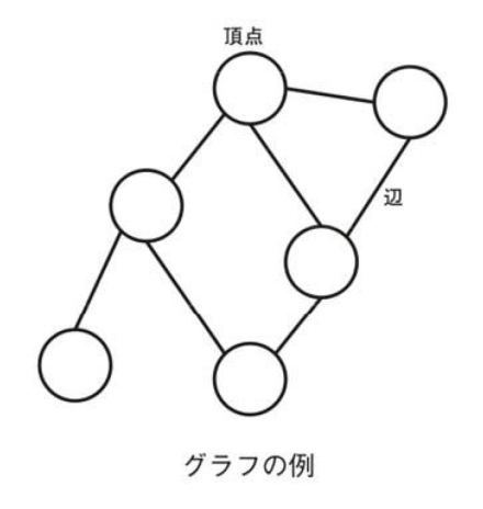
A graph consists of vertices (vertex, node) and edges (edge). A vertex represents an object, which is pictured as a point or a circle in a diagram. An edge represents a connection between two objects, and is drawn as a line segment connecting two points in the figure. A graph whose set of vertices is V and whose set of edges is E is denoted by G=(V,E), and the edge connecting two points u and v is denoted by e=(u,v).

There are two main types of graphs. A graph with no edge orientation is called an undirected graph, and a graph with edge orientation is called a directed graph. A graph of friendships (with people as vertices and friendships as edges) or a route map is an undirected graph, while a graph of numbers (with numbers as vertices and edges drawn from A to B when A>B) or a flowchart is a directed graph.

Various attributes can be attached to edges. A typical example is cost. A graph with weights attached to edges is called a weighted graph. Weights can be interpreted in various ways depending on the problem, such as distance, time, or price.
When there is an edge between two vertices, we say that the two vertices are adjacent. A sequence of adjacent vertices is called a path. A path whose start and end points are the same is called a closed path. A graph in which a path exists between any two vertices is called a connected graph. The number of edges connected to a vertex is called the degree of that vertex.

A connected graph with no closed paths is called a tree, and an unconnected graph with no closed paths is called a forest. A tree has the number of edges exactly equal to vertex -1. A connected graph with the number of edges equal to vertex -1 is a tree.

If you choose one vertex, called the root, you can arrange the tree so that the root is at the top and the vertices farther from the root are at the bottom. This kind of tree is called a clubbed tree. A normal tree that is not a clubbed tree can also be made into a clubbed tree by choosing the appropriate vertex to make it easier to handle. If we look at a cudgel tree as a family tree, we can give a parent-child relationship between the vertices. This can also be thought of as giving an orientation to the edges.

For a vertex v of a directed graph, we denote by δ+(v) the set of edges going out of v and by δ-(v) the set of edges coming in. We call |δ+(v)| the outgoing degree of v and |δ-(v)| the incoming degree.
A directed graph with no closed paths is called a DAG (Directed Acyclic Graph). For example, if we consider a graph with an integer as a vertex and an edge from n to m when n divides m, this is a DAG. As in this case, an ordering relation can be given between the vertices of a DAG.

Assign a number to the extension points and let the i-th vertex be vi. When there is an edge from vertex vi to vertex vj, the numbering scheme such that i<j holds is called topological ordering.

If we rearrange the vertices from left to right according to the topological ordering, all edges will be left to right. This kind of ordering can sometimes be used to solve DAG problems using DP. Finding the topological ordering is called topological sorting.
In order to handle graphs programmatically, it is necessary to have vertices and edges as concrete data. Two typical ways of representing graphs are adjacency matrices and adjacency lists. Both representations have advantages and disadvantages, and depending on the problem, some of them may affect the amount of computation. Let V and E be a set of vertices and edges, and let|V|and|E|be the number of vertices and edges. Also, assume that V is numbered from 0 to|V|-1.
First, let’s look at the adjacency matrix. In the adjacency matrix, the graph is represented by a two-dimensional array g of |V|x|V|, where g[i][j] represents the relationship between the i-th and j-th vertices.
In the case of an undirected graph, we only need to know whether the i-th and j-th vertices are connected by an edge, so we can represent an undirected graph by setting the values of g[i][j] and g[j][i] to 1 if vertex i and vertex j are connected by an edge, and 0 otherwise.

In the case of a directed graph, we only need the information “whether there is an edge from vertex i to vertex j”, so we can represent a directed graph by setting the value of g[i][j] to 1 if there is an edge from vertex i to vertex j, and 0 otherwise. In this case, unlike the undirected graph, g[i][j] ≠ g[j][i].

In the case of a weighted graph, let g[i][j] be the weight of the edge from vertex i to vertex j. If there is no edge, putting 0 or more will be indistinguishable from the case where the weight is 0. If there is no edge, the weight of g[i][j] is indistinguishable from the weight of 0, so we define an appropriately large (whatever is distinguishable) constant INF, and set g[i][j]=INF. Of course, if it is an undirected graph, g[i][j]=g[j][i]. If you have several attributes, you can handle them in the same way by preparing several arrays of |V|x|V| or by using structures or classes for the elements of the arrays.

The advantage of the adjacency matrix is that it can determine whether there is an edge between two vertices in a constant time, but it always consumes O(|V|2) memory without fail. However, it always consumes O(|V|2) memory. If there are few edges, a large amount of space is wasted. For example, if we consider a tree, the number of edges is exactly |V|-1, which means that most of the elements of the array g are filled with zeros. For example, if the number of edges is exactly|V|-1, then most of the elements of array g are filled with zeros, and if|V| is 1000000, then even if the element of g is one byte, the memory is nearly 1TB of evidence.
Also, care must be taken when there are multiple edges and accidental loops.

In the unweighted case, it is enough to put the number of edges from vertex i to vertex j in g[i][j], but in the weighted case, it becomes more complicated. In most cases, it is enough to have the smallest (largest) weight and ignore the rest. However, if you really want to keep multiple edges, use the adjacency list described next.
In the case of an adjacency matrix, if the number of variables is small, memory is consumed unnecessarily, but in the case of an adjacency list, the graph is represented by having information such as “there is an edge from vertex 0 to vertices 2, 4, and 5” as a list. In this case, only O(|V|+|E|) consumes memory.

There are various ways to implement an adjacency list in practice. When edges have attributes, such as weighted graphs, it is easier to manage and consume less memory to create a structure or class representing the edges.
These graph structures can be used to solve problems such as search problems, bipartite graph decision (coloring), shortest distance, and minimum total area trees. Algorithms that combine machine learning techniques are also being used. These are listed below.
Implementation in machine learning
SNAP is an open-source software library developed by the Computer Science Laboratory at Stanford University that provides tools and resources used in various network-related studies, including social network analysis, graph theory, and computer network analysis. The library provides tools and resources used in a variety of network-related research, including social network analysis, graph theory, and computer network analysis.
CDLib (Community Discovery Library) is a Python library that provides community detection algorithms, offering a variety of algorithms for identifying community structure in graph data and helping researchers and data scientists address different It will support researchers and data scientists in dealing with different community detection tasks.
MODULAR is one of the methods and tools used in the research areas of computer science and network science to solve multi-objective optimization problems of complex networks, the approach is designed to simultaneously optimize the structure and dynamics of the network, taking different objective functions ( multi-objective optimization) are taken into account.
The Louvain method (or Louvain algorithm) is one of the effective graph clustering algorithms for identifying communities (clusters) in a network. The Louvain method employs an approach that maximizes a measure called modularity to identify the structure of the communities.
Infomap (Information-Theoretic Modularity) is a community detection algorithm used to identify communities (modules) in a network. It focuses on optimizing the flow and structure of information.
Copra (Community Detection using Partial Memberships) is an algorithm and tool for community detection that takes into account the detection of communities in complex networks and the fact that a given node may belong to multiple communities. Copra is suitable for realistic scenarios where each node can belong to multiple communities using partial community membership information.
IsoRankN is one of the algorithms for network alignment, which is the problem of finding a mapping of corresponding vertices between different networks. IsoRankN is an improved version of the IsoRank algorithm that maps vertices between different networks with high accuracy and efficiency. IsoRankN aims to preserve similarity in different networks by mapping vertices taking into account their structure and characteristics.
- Overview of the Weisfeiler-Lehman Algorithm, Related Algorithms, and Examples of Implementations
The Weisfeiler-Lehman Algorithm (W-L Algorithm) is an algorithm for graph isomorphism testing and is primarily used to determine whether two given graphs are isomorphic.
Techniques for analyzing graph data that changes over time have been applied to a variety of applications, including social network analysis, web traffic analysis, bioinformatics, financial network modeling, and transportation system analysis. Here we provide an overview of this technique, its algorithms, and examples of implementations.
Snapshot Analysis (Snapshot Analysis) is a method of data analysis that takes into account changes over time by using snapshots of data at different time points (instantaneous data snapshots). This approach helps analyze data sets with information about time to understand temporal patterns, trends, and changes in that data, and when combined with Graphical Data Analysis, allows for a deeper understanding of temporal changes in network and relational data. This section provides an overview of this approach and examples of algorithms and implementations.
Dynamic Community Detection (Dynamic Community Analysis) will be a technique for tracking and analyzing temporal changes in communities (modules or clusters) within a network with time-relevant information (dynamic network). Usually targeting graph data (dynamic graphs) whose nodes and edges have time-related information, the method has been applied in various fields, e.g., social network analysis, bioinformatics, Internet traffic monitoring, financial network analysis, etc. It is used in the following areas.
Dynamic Centrality Metrics is a type of graph data analysis that takes into account changes over time. Usual centrality metrics (e.g., degree centrality, mediation centrality, eigenvector centrality, etc.) are suitable for static networks and It provides a single snapshot of the importance of a node. However, since real networks often have time-related elements, it is important to consider temporal changes in the network.
Dynamic module detection is a method of graph data analysis that takes time variation into account. This method tracks changes in communities (modules) in a dynamic network and identifies the community structure at different time snapshots. Here we present more information about dynamic module detection and an example implementation.
Graph data analysis that takes into account changes over time using a time prediction model is used to understand temporal patterns, trends, and predictions in graphical data. This section discusses this approach in more detail.
Tensor decomposition (TD) is a method for approximating high-dimensional tensor data to low-rank tensors. This technique is used for data dimensionality reduction and feature extraction and is a useful approach in a variety of machine learning and data analysis applications. The application of tensor decomposition methods to dynamic module detection is relevant to tasks such as time series data and dynamic data module detection.
MAGNA is a set of algorithms and tools for mapping different types of nodes (e.g., proteins and genes) in biological networks. This approach can be useful for identifying relationships between different types of biological entities.
TIME-SI (Time-aware Structural Identity) is one of the algorithms or methods for identifying structural correspondences between nodes in a network, taking into account time-related information. It will be used in a variety of network data, including social networks.
Diffusion Models for graph data is a method for modeling how information and influence spread over a network, and is used to understand and predict the propagation of influence and diffusion of information in social networks and network structured data. Below is a basic overview of Diffusion Models for graph data.
GRAAL (Graph Algorithm for Alignment of Networks) is an algorithm to align different network data, such as biological networks and social networks, and is mainly used for comparison and analysis of biological networks. GRAAL is designed to solve network mapping problems and identify common elements (nodes and edges) between different networks.
HubAlign (Hub-based Network Alignment) is an algorithm for mapping (alignment) between different networks, which is used to identify common elements (nodes and edges) between different networks. It is mainly used in areas such as bioinformatics and social network analysis.
IsoRank (Isomorphism Ranking) is an algorithm for aligning different networks, which uses network isomorphism (graph isomorphism) to calculate the similarity between two different networks and estimate the correspondence of nodes based on it. IsoRank is used in areas such as data integration between different networks, network comparison, bioinformatics, and social network analysis.
- Overview of DynamicTriad and Examples of Algorithms and Implementations
DynamicTriad is a method for modeling temporal changes in dynamic graph data and predicting node correspondences. This approach has been applied to predicting correspondences in dynamic networks and understanding temporal changes in nodes.
- Overview of MODA (MOdule Detection in Dynamic Networks Algorithm) and Examples of Implementations
MODA is an algorithm for detecting modules (groups of nodes) in dynamic network data. MODA will be designed to take into account changes over time and to be able to track how modules in a network evolve. The algorithm has been useful in a variety of applications, including analysis of dynamic networks, community detection, and evolution studies.
- DynamicTriad Overview, Algorithm and Implementation Examples
DynamicTriad is one of the models used in the field of Social Network Analysis (SNA), a method to study the relationships among people, organizations, and other elements and to understand their network structure and characteristics. Network Analysis Using Clojure (2) Calculating Triads in a Graph Using Glittering”, DynamicTriad is a tool for understanding the evolution of an entire network by tracking changes in a triad (set of triads) consisting of three elements. This approach allows for a more comprehensive analysis of the network, since it can take into account not only the individual relationships within the network, but also the movements of groups and subgroups.
- Overview of the Girvan-Newman Algorithm and Examples of Implementations
The Girvan-Newman algorithm is an algorithm for detecting the community structure of a network in graph theory, By removing these edges, the network is partitioned into communities.
Subsampling of large graph data reduces data size and controls computation and memory usage by randomly selecting portions of the graph, and is one technique to improve computational efficiency when dealing with large graph data sets. In this section, we discuss some key points and techniques for subsampling large graph data sets.
Displaying and animating graph snapshots on a timeline is an important technique for analyzing graph data, as it helps visualize changes over time and understand the dynamic characteristics of graph data. This section describes libraries and implementation examples used for these purposes.
- Graph data analysis that takes into account temporal variation with network alignment
Network alignment is a technique for finding similarities between different networks or graphs and mapping them together. By applying network alignment to graph data analysis that takes into account temporal changes, it is possible to map graphs of different time snapshots and understand their changes.
This paper describes the creation of animations of graphs by combining NetworkX and Matplotlib, a technique for visually representing dynamic changes in networks in Python.
Methods for plotting high-dimensional data in low dimensions using dimensionality reduction techniques to facilitate visualization are useful for many data analysis tasks, such as data understanding, clustering, anomaly detection, and feature selection. This section describes the major dimensionality reduction techniques and their methods.
Gephi is an open-source graph visualization software that is particularly suitable for network analysis and visualization of complex data sets. Here we describe the basic steps and functionality for visualizing data using Gephi.
Cytoscape.js is a graph theory library written in JavaScript that is widely used for visualizing network and graph data. Cytoscape.js makes it possible to add graph and network data visualization to web and desktop applications. Here are the basic steps and example code for data visualization using Cytoscape.js.
- Visualization of Graph Data Using Sigma.js
Sigma.js is a web-based graph visualization library that can be a useful tool for creating interactive network diagrams. Here we describe the basic steps and functions for visualizing graph data using Sigma.js.
- Overview of Bayesian Neural Networks and Examples of Algorithms and Implementations
Bayesian neural networks (BNNs) are architectures that integrate probabilistic elements into neural networks, whereas regular neural networks are deterministic, BNNs build probabilistic models based on Bayesian statistics. This allows the model to account for uncertainty and has been applied in a variety of machine learning tasks.
The Page Rank Algorithm, invented by Google co-founder Larry Page, is an algorithm used to calculate the importance of a web page. It is this innovation in search technology using the Page Rank algorithm that has propelled Google to its current position. Page rank technology is one of the elemental technologies used in search engines to rank search results. This section provides an overview of this page rank algorithm and examples of its implementation.
Similarity is a concept that describes the degree to which two or more objects or things have common features or properties and are considered similar to each other, and plays an important role in evaluating, classifying, and grouping objects in terms of comparison and relatedness. This section describes the concept of similarity and general calculation methods for various cases.
- Directed Acyclic Graphs and Blockchain Technology
Directed Acyclic Graph (DAG) is a graph data algorithm that appears in various situations such as automatic management of various tasks and compilers. In this article, I would like to discuss DAGs.
Relational Data Learning is a machine learning method for relational data (e.g., graphs, networks, tabular data, etc.). Conventional machine learning is usually applied only to individual instances (e.g., vectors or matrices), but relational data learning considers multiple instances and the relationships among them.
This section discusses various applications for this relational data learning and specific implementations in algorithms such as spectral clustering, matrix factorization, tensor decomposition, probabilistic block models, graph neural networks, graph convolutional networks, graph embedding, and metapath walks. The paper describes.
A knowledge graph is a graph structure that represents information as a set of related nodes (vertices) and edges (connections), and is a data structure used to connect information on different subjects or domains and visualize their relationships. This paper outlines various methods for automatic generation of this knowledge graph and describes specific implementations in python.
A knowledge graph is a graph structure that represents information as a set of related nodes (vertices) and edges (connections), and is a data structure used to connect information on different subjects or domains and visualize their relationships. This section describes various applications of the knowledge graph and concrete examples of its implementation in python.
Structural Learning is a branch of machine learning that refers to methods for learning structures and relationships in data, usually in the framework of unsupervised or semi-supervised learning. Structural learning aims to identify and model patterns, relationships, or structures present in the data to reveal the hidden structure behind the data. Structural learning targets different types of data structures, such as graph structures, tree structures, and network structures.
This section discusses various applications and concrete implementations of structural learning.
GraphX will be a distributed graph processing library designed to work in conjunction with Spark. Like the MLlib library described in “Large-scale Machine Learning with Apache Spark and MLlib,” GraphX provides a set of abstractions built on top of Spark’s RDDs. By representing graph vertices and edges as RDDs, GraphX can handle very large graphs in a scalable manner.
By restricting the types of computations that can be represented and introducing techniques for partitioning and distributing graphs, graph parallel systems can execute sophisticated graph algorithms several orders of magnitude faster and more efficiently than typical data parallel systems.
The Pregel API will be the primary abstraction in GraphX for representing custom, iterative graph parallel computing. It is named after Google’s 2010 in-house system for performing large-scale graph processing. It is also the name of the river over which the famous Königsberg bridge spans in the problem of Euler paths (paths through all edges of a graph) in graphs, described in “Network Analysis Using Clojure (1) Width-first/Depth-first Search, Shortest Path Search, Minimum Spanning Tree, Subgraphs and Connected Components”.
Google’s Pregel paper popularized the “think like a vertex” approach to graph parallel computing; Pregel’s model essentially uses message passing between graph vertices organized into a series of steps, called supersteps. At the beginning of each superstep, Pregel executes a user-specified function on each vertex, passing on all messages sent to that vertex in the previous superstep. The vertex function has the opportunity to process each of these messages and send messages to other vertices in turn. A vertex may also “vote to stop” the computation, and if all vertices vote to stop, the computation is terminated.
In the previous section “Network Analysis with GraphX Pregel using Clojure Glittering”, we discussed whether it is possible to identify what connects the largest communities among those analyzed in the previous section “Network Analysis with GraphX Pregel using Clojure Glittering”. There are various ways to do this. If we had access to the tweets themselves, we could perform textual analysis, as we do with clustering, to see if certain words or certain languages are used more frequently among these groups.
In this section, we discuss network analysis. There, the graph structure is used to identify the most influential accounts in each community. This means, for example, that a list of the top 10 most influential accounts would be an indicator of what resonates with their followers.
D3.js and React, which are based on Javascript, can be used as tools for visualizing relational data such as graph data. In this article, we will discuss specific implementations using D3 and React for 2D and 3D graph displays, and heat maps as a form of displaying relational data.
- Techniques for displaying and animating graph snapshots on a timeline
Displaying and animating graph snapshots on a timeline is an important technique for analyzing graph data, as it helps visualize changes over time and understand the dynamic characteristics of graph data. This section describes libraries and implementation examples used for these purposes.
Graph Neural Network
Graph neural networks (GNNs) apply deep learning to graph data, extracting features from the data, constructing neural networks based on the feature representations, and connecting them in multiple stages to capture complex data patterns and construct models with nonlinearities. The following is a comparison of the two types of neural networks.
The difference between ordinary deep learning and graph neural networks is that ordinary deep learning uses a grid-like data structure of image data, text data, etc., and calculates them based on matrix operation algorithms, while GNN specializes in graph structures and calculates data represented by a combination of nodes and edges GNN specializes in graph structures and computes data represented by a combination of nodes and edges.
In the following pages of this blog, the algorithm, implementation examples, and various application examples of GNN are described.
Basic Graph Data Algorithm
- Fundamentals of Graph Network Algorithms
- Introduction to Graph Theory
- What is a Complex Network? A New Approach to Deciphering Complex Relationships Reading Memo
“My friend’s ex-boyfriend was my ex-boyfriend!” A small world where you can reach anyone in the world just by tracing six people. Complex networks” is the biggest keyword of the 21st century. By applying the concept of “complex networks,” we can replace the seemingly complicated phenomena around us with simple relationships. You will discover “surprising rules” in the infection routes of infectious diseases and computer viruses, the way neurons and proteins transmit information, and human relationships in companies and society.
Consider the case where graphs are treated in a mathematical rather than a visual sense. A graph is simply a set of vertices connected by edges, and the simplicity of this abstraction means that graphs can be anywhere. Graphs are valid models for a variety of structures, including the hyperlink structure of the Web, the physical structure of the Internet, roads, telecommunications, and social networks.
For these graph data algorithms, we have previously described C++ implementations of “basic algorithms for graph data (DFS, BFS, bipartite graph decision, shortest path problem, minimum global tree)” and “advanced graph algorithms (strongly connected component decomposition, DAG, 2-SAT, LCA)”. In this article, we will discuss the use of Clojure/loop.
- Graph Clustering (external link)
- Basic algorithms for graph data (DFS, BFS, bipartite graph decision, shortest path problem, minimum-wide tree)
A subset S of vertices of an effective graph is said to be strongly connected if it satisfies the condition “for any two vertices u and v, u can be reached from v”. We say that S is a Strongly Connected Component (SCC) if no other vertex set can be added to the strongly connected set of vertices S to make it strongly connected. Any directed graph can be decomposed into a union of several strongly connected components that have no common part. This is called strongly connected component decomposition. By collapsing the strongly connected components into a single vertex, we get a DAG (directed graph without closed paths).
Given a logical formula, the problem of determining whether the entire formula can be made true by appropriately assigning boolean values to its logical variables is called the satisfiability problem (SAT). solving SAT is generally NP-complete, but it can be solved efficiently if there are restrictions on the form of the logical formula.
For a rooted tree, the nearest common ancestor of its vertices u and v is called the Lowest Common Ancestor (LCA) of u and v. There are various methods to find the LCA efficiently, and we will discuss two methods here.
We will discuss graphical flows (flows), focusing on maximum and minimum cost flows. Flows have a variety of properties and applications and are widely used. In this talk, we will discuss the Ford-Fulkerson algorithm for solving the maximum communication problem and its relation to the minimum cut problem, the maximum matching problem for nipartite graphs, which is a special case of the maximum flow problem, the general matching problem and the minimum cost flow problem.
Submodular functions can be minimized efficiently. In particular, minimization of cut functions of directed graphs can be performed by the maximum flow algorithm, which is theoretically/practically fast. In this section, we discuss the basics of the maximum flow algorithm, and as an example of what is attributed to such a computation, we discuss inference over Markovian stochastic fields, and describe a class of fast computationally feasible submodular functions that are often used in practical applications.
Graph cutting is known to be an algorithm that can be applied to problems on the order of tens of thousands to millions in practical time, but in terms of the submodular functions, it can be interpreted as minimizing the cut function, which is roughly a second-order submodular function. It is known that a theoretically/practically fast algorithm called the maximum flow algorithm can be applied to the minimization of the cut function. Whether or not it can be described as such a minimization of the cut function is one way to measure whether or not the combinatorial computation can be performed in a practical manner.
In order to understand this relationship, we will first look at the relationship between the minimization of the cut function and the calculation of the maximum flow in a network, and then look at a concrete method for actually performing the maximum flow calculation.
In this issue, we will discuss the flow increment method, which is a typical algorithm for finding the maximum flow, and we will also discuss how to calculate the minimum s-t cut using the maximum flow algorithm and the proof of the maximum flow minimum cut theorem. We also describe the Bliflow-Bush method, a fast maximum flow algorithm based on a different principle from the flow incremental method.
When dealing with multivariate data, if each variable in the data has some structure, various inference algorithms may be described recursively using that structure. The Markov probability field is a typical model, which uses an undirected graph to represent Markovianity among variables. In this section, we discuss the relationship between the maximum-a-posteriori estimation (maximum-posteriori estimation) of a Markov random field and column-reduced modular optimization. Furthermore, we discuss how graph cuts, which are widely used in computer vision and other fields, are essentially minimizing s-t cuts.
As mentioned above, the s-t cut function of a directed graph is a special class of submodular functions that can be minimized quickly. However, of course, this function alone is not sufficient in various practical situations due to its limited descriptive power. Therefore, it would be extremely useful in practical situations if a function could be devised that is more descriptive than the s-t cut function for directed graphs and can be minimized as fast as this function. Here, we discuss graph-representable submodular functions as one answer to this question. Graph-representable submodular functions are functions that can be represented as s-t cut functions of directed graphs by adding some auxiliary vertices, and are a class of practically useful functions as described above.
Next, we discuss the pre-flow push method as a method to compute the maximum flow for minimizing the s-t cut function of a directed graph. As mentioned above, a computationally O(nm) algorithm by Orlin has recently been proposed for the maximum flow. In the case of the pre-flow push method, the computational complexity is O(mnlogn2/m), but it is still an important algorithm for applications because of its known fast implementation in practical use. The method can also be extended to parametric optimization, which will also play an important role in the following section.
The feasible flows were such flows ξ = (ξe)e∈ℰ that satisfy both the “capacity constraint” and the “flow conservation constraint”. In the preflow-push method, instead of the feasible flow, a flow called preflow, which is obtained by relaxing the flow conservation constraints, is considered, and the maximum flow is calculated by iteratively updating this preflow to gradually satisfy the flow conservation speed and finally obtaining the feasible flow.
- Decision Tree Algorithm (1) Overview
A decision tree learner is a powerful classifier that uses a tree structure to model the relationship between possible outcomes as futures.
A key feature of the decision tree algorithm is that the flowchart-like tree structure is not necessarily exclusive to the learner, but the output results of the model can be read by humans to provide a great hint as to why or how the model does (or does not) work well for a particular task.
Such a mechanism can be particularly useful when the classification mechanism must be transparent for legal reasons, or when the results are shared with others to make explicit business practices between organizations.
- Decision Tree Algorithm (2) Clustering with R
In this article, we will discuss clustering of decision trees using R.
The data to be used is the bank.zip of the Bank Marketing Data Set, which is downloaded from the machine learning data repository of the University of Hamburg. This data set contains data from a financial credit survey in Germany.
- Decision Tree Algorithm (3) Rules extraction
Classification rules represent knowledge in the form of logical if-else statements that give classes to unlabeled instances. These are designated as “antexedent” and “consequent,” and form the hypothesis that “if this happens, that happens. A simple rule asserts something like, “If the hard disk is ticking, it will soon make an error. The prior case consists of a specific combination of feature values, whereas the posterior case specifies the class values that will be given when the conditions of the rule are met.
Classification rule learning is often used in the same way as decision tree learning. Classification rules can be specifically used in applications that generate knowledge for future actions, such as the following. (1) identifying conditions that cause hardware errors in mechanical devices, (2) describing key characteristics of groups of people belonging to customer segments, (3) extracting conditions that herald a significant drop or rise in stock market prices.
- Decision Tree Algorithm (4) Rule Extraction in R
In this article, we will discuss the extraction of rules using decision trees with R.
As in the previous article, we will use the same data from the UCI repository to extract the rules: “Is the mushroom edible? Is it poisonous? from the UCI repository.
In this article, we describe an algorithm for learning how to sort alignments by presenting many correct alignments (positive examples) and incorrect alignments (negative examples). The main difference between these approaches is that the techniques in this section require some sample data for learning. This can be provided by the algorithm itself, such as providing only a subset of the correspondences to be judged, or it can be determined by the user or brought from an external resource.
What is topological sorting?
A sequence of vertices with the following properties 𝑣1, 𝑣2, … , 𝑣𝑛
– For all edges 𝑣𝑖, 𝑣𝑗, 𝑖 < 𝑗
– In other words, all edges face “forward” in that order
Graph Data Visualization Technology
D3.js and React, which are based on Javascript, can be used as tools for visualizing relational data such as graph data. In this article, we will discuss specific implementations using D3 and React for 2D and 3D graph displays, and heat maps as a form of displaying relational data.
Theory and application of combination with machine learning technology
Sparse modeling is a technique that takes advantage of sparsity in the representation of signals and data. Sparsity refers to the property that non-zero elements in data or signals are limited to a very small portion. The purpose of sparse modeling is to efficiently represent data by utilizing sparsity, and to perform tasks such as noise removal, feature selection, and compression.
This section provides an overview of sparse modeling algorithms such as Lasso, compression estimation, Ridge regularization, elastic nets, Fused Lasso, group regularization, message propagation algorithms, dictionary learning, etc., as well as a description of the various algorithms used in image processing, natural language processing, recommendation, signal processing The paper describes the implementation of the algorithms in various applications such as image processing, natural language processing, recommendation, machine learning, signal processing, brain science, and so on.
- Graphical models (1) Bayesian network
Graphical models are probabilistic models described using graphs. Probabilistic models introduce “uncertainty” into the events handled in machine learning, some of which are inherently unstable, and some of which are caused by a simple lack of information.
The basic concept of a probabilistic model is to connect these uncertain events (random variables) with edges that show relationships between them to form a graph. These are often utilized in scenes representing complex models in machine learning.
- Graphical models (2) Markov probability field
A Bayesian network is a probability field in which one random variable determines another random variable, whereas a Markov probability field is a model in which the random variables are interrelated.
The simplest Markov probability model is called the Ising model. This model is used in physics as a model for magnetic materials, and has a lattice of +/- values called spins (+1 for spin pointing up, -1 for spin pointing down), as shown below.
- Clustering of symmetric relational data spectral clustering
Spectral clustering is a typical method for object clustering of target relational data (unoriented, single-domain relational data). This method is mainly applied to the task of community detection. A community is a cluster in which objects are tightly coupled within the cluster and very loosely coupled with objects in another cluster, also called an assortative cluster. Conversely, a cluster that is loosely coupled within a cluster and tightly coupled to the outside is called a disassortative cluster.
- Clustering Techniques for Asymmetric Relational Data – Probabilistic Block Model and Infinite Relational Model
The goal of the Stochastic Block Model (SBM) is “relational data clustering that can be applied to asymmetric data and can extract clusters other than tightly coupled clusters. Here, SBM uses a generative “stochastic model” approach that assumes the existence of a “potential block structure”.
- Matrix factorization -Extraction of relational features between two objects
As an example of matrix decomposition, consider the task of recommending movies where customers are the rows, movies are the columns, and the element values are the ratings; with a huge number of users such as Netflix, it would be difficult to store and process this matrix at its original scale. The solution to this problem is data compression.
- Higher-order relational data – Overview of tensor data processing
In this article, we will discuss the relationship between three or more objects. As an example, let’s consider expressing the evaluation of a movie as a ternary relationship of “customer, movie, and time.
Other examples include: meteorological data, where locations on the earth are represented by latitude and longitude, and various measurements such as wind speed, temperature, and humidity are collected at each observation point, and analyzed as “latitude, longitude, and measurement”; and linguistic data, where information such as “a certain verb tends to appear with a certain subject or object” can be obtained by counting the frequency of three combinations of subject, verb, and object in each sentence of multiple documents.
- Tensor decomposition – CP decomposition and Tucker decomposition
Tensor decomposition has the property that the number of elements can easily increase compared to matrices. When the order of all modes is the same (I=J=K>1), the number of elements in a matrix is I2, while the number of elements in a third-order tensor is I3 and that of an L-order tensor is IL. As you can see, the higher the order, the more rapidly the number of elements increases even if I is small. Intuitively, we can use the idea of dimensional compression, which we have seen in matrix factorization, to handle this kind of large scale well.
For simplicity, let us assume that the number of characters in the tensor is 3, and the data is a tensor χ with size IxJxK. In the dimensional compression of matrices, it is assumed that each row vector of the matrix is represented in a lower dimensional space. We consider a “mode 1 slice” as corresponding to a “row vector” in the tensor. In this way, dimensional compression in tensors can be regarded as “the representation of each mode 1 slice as a vector in a lower dimensional space. Since “mode 1 slices” are matrices, we need to map vectors to matrices in order to consider this dimensional compression.
- Anomaly detection using Gaussian process regression -Output anomaly detection for input, application to design of experiments
This paper describes an anomaly detection technique for systems where input-output pairs can be observed. In this case, the relationship between input and output is modeled in the form of a response surface (or regression curve), and anomalies are detected in the form of deviations from the response surface. In practical use, the relationship between input and output is often non-linear. In this article, we will discuss the Gaussian process regression method, which has a wide range of engineering applications among the nonlinear regression techniques.
When both input and output are observed, the most natural way to detect anomalies is to look at the output for a given input and see if it deviates significantly from the value expected by normal behavior. In this sense, this problem can be called a response anomaly detection problem.
- Change detection using subspace method -Singular spectral transform method for time series data
This paper discusses the problem of change detection with time series data in mind. Change detection cannot be achieved simply by calculating the degree of anomaly of a single sample. In this paper, we first describe the concept of cumulative sum and sliding window as the basic techniques to combine multiple anomalies or samples, and then abstractly formulate the change detection as a sequential density estimation problem. As the simplest concrete example, I describe a change detection method called the singular spectral transformation method. The singular spectral transform method is one of the most important change detection methods in practice because of its versatility and robustness against noise.
First, I will discuss the cumulative summation method, which is a classical change detection technique. As an example, suppose we are monitoring the concentration of a particular chemical substance in a reactor of a chemical plant from time to time. Since chemicals come and go as fluids, it is inevitable that the concentration may be high or low locally, and in this case, a monitoring technique such as Hotelling’s T2 method, which calculates the degree of anomaly for each observation, is inappropriate. In this case, what we want to do is to detect whether or not some abnormal situation is occurring continuously, in other words, change detection, rather than a sudden and unexpected abnormal value.
When the data is given as a pair of scalar output y and M-dimensional vector x, D={(y(n),x(n))|n=1,…,N}, we will discuss how to achieve a sparse solution as a linear regression (sparsifying the regression coefficients, or sparsifying in the sense of eliminating extra samples rather than variables).
As a use case, I will discuss the case where the observed data is contaminated with noise and not all samples can be trusted, as well as the case where a machine is constantly monitored by a fixed number of sensors by extending it to graph data.
- Graph Neural Networks (1) Overview
An overview of graph neural network technology, a framework for performing deep learning on graph data. It is used for estimating physical properties of compounds, natural language processing using Attension, co-occurrence networks, and image information processing.
The quasi-Newton method avoids the computation of the Hesse matrix in the Newton method and provides an efficient optimization method. In this article, we will review typical algorithms, describe their relation to geometric structures on the positive definite matrix space, and discuss how to utilize the sparsity of the Hesse matrix.
Application to knowledge graphs, etc.
A Knowledge Graph is a representation of information in the form of a graph structure, which will play an important role in the field of Artificial Intelligence (AI). Knowledge graphs are used to represent the knowledge that multiple entities (e.g., people, places, things, concepts, etc.) have relationships between them (e.g., “A owns B,” “X is part of Y,” “C affects D,” etc.).
Specifically, knowledge graphs play an important role in search engine question answering systems, artificial intelligence dialogue systems, and natural language processing. These systems can use knowledge graphs to efficiently process complex information and provide accurate information to users.
RDF (Resource Description Framework) is a technical framework for the metadata of resources on the Web, which was standardized by W3C in February 1992, as mentioned in LOD.
The structure of RDF is based on the triple data model. The structure of RDF is based on the triple data model, which expresses relational information about resources using three elements: subject, predicate, and object.
The composite similarity calculation is still local, since it only considers the neighborhood of a node to provide similarity. However, the similarity is for the entire ontology, and the final similarity value may ultimately depend on all ontology entities. Furthermore, if the ontology is not reduced to a directed acyclic graph, distances defined in a local manner may be defined in a circular manner. This is the most common case. It occurs, for example, when the distance between two classes depends on the distance between instances that depend on the distance between those classes, or when there is a circulation in the ontology. As shown in the figure below, the similarity between Product and Book depends on the similarity between hasProvider and hasCreator and author, publisher, and translator. And the similarity between these elements ultimately depends on the similarity between Product and Book. The two graphs are homo morphic in many ways.
The next best known structure after Taxonomic (taxonomic) structure would be the mereologic (part-whole) structure, that is, the structure corresponding to the part-of relationship: the two classes Book and Volume are found to be equivalent, suggesting that the two classes InBook and BookChapter, respectively, suggesting that if there is a mereologic relationship between the classes InBook and BookChapter, the two classes may be related as well. This inference also applies in the reverse direction, from the part to the whole. This is the case when there are separate parts, i.e., when the parts of a journal Issue are distinguished into editporial, article, recessions, and letture.
The difficulty in dealing with such a structure is that it is not easy to find properties that have just a structure. For example, the Proceedings class can have several whole-part relationships with the InProceedings class, which are represented by properties communications. These InProceedings objects would then have just a structure represented by section properties.
Many people accept the fact that natural language sentences convey some kind of information, i.e., meaning. However, when asked “What is meaning?” or “How do you define it on a computer (or in mathematical terms)?” few people, even natural language experts, can answer clearly. The meaning of natural language becomes a kind of dark matter that is almost certain to exist but that no one has ever seen.
- Application of Knowledge Graphs to Question and Answer SystemsA knowledge graph can be defined as “a graph created by describing entities and the relationships among them. Entities” here are things that “exist” physically or non-physically and are not necessarily material entities, but are abstracted to represent things (events in mathematics, law, academic fields, etc.).Examples of knowledge graphs include simple and concrete things such as “there is a pencil on the table” and “Mt. Fuji is located on the border between Shizuoka and Yamanashi prefectures,” as well as more abstract things such as “if a=b, then a+c = b+c,” “the consumption tax is an indirect tax that focuses on “consumption” of goods and services,” “in electronically controlled fuel injection systems In the case of electronically controlled fuel injection systems, the throttle chamber is an intake throttling device that is attached to the collector of the intake manifold and contains a throttle valve to control the amount of intake air.The advantage of using these knowledge graphs, from AI’s perspective, is that machines can access the rules, knowledge, and common sense of the human world through the data in the knowledge graphs. In contrast to the recent black-box approaches, such as deep learning, which require a large amount of teacher data in order to achieve learning accuracy, AI can produce results that are easy for humans to interpret, and AI can generate data based on knowledge data to enable machine learning with small data. Machine learning with small data is possible by generating data based on knowledge data.By applying this knowledge graph to question-answer systems, it is possible to create a hierarchical structure of key terms, rather than simple FAQ question-answer pairs, and further associate them with context-specific questions and their alternatives, synonyms, and machine-learned response classes to provide an intelligent FAQ experience. It is possible to provide an intelligent FAQ experience.

コメント