Machine Learning Artificial Intelligence Digital Transformation Probabilistic Generative Models Deep Learning Nonparametric Bayesian and Gaussian processes Support Vector Machine Clojure Navigation of this blog
What is Gaussian process?
A Gaussian process is like a box (stochastic process) that randomly outputs a function form. For example, if we consider that the process of a dice generating the natural numbers 1, 2, 3, 4, 5, and 6 depends on the distortion of the dice, we can think that the appearance of the function ( The function representing the probability that the dice will turn up) will change depending on the parameters (in this case, the distortion of the dice).
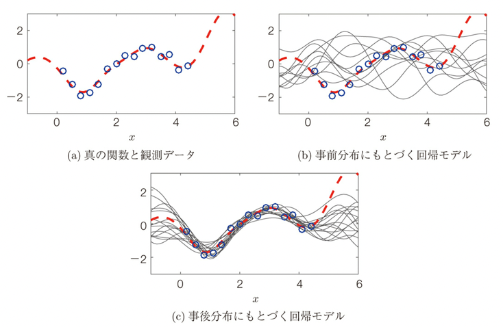
As an example of Gaussian process regression, when the functional relationship between input x and output y (red dotted line) and the observed data (blue circled line) for a part of it are obtained, this functional relationship can be expressed as follows using the Gaussian process, where the random cloud-like distribution in the prior distribution converges when real data is given.

Using such a Gaussian process (cloud of functions) provides advantages not found in other machine learning such as (1) when a cloud of functions is obtained, the degree of unknowability is known, (2) when a cloud of functions is obtained, the difference between confident and unconfident regions is known, (3) when a cloud of functions is obtained, model selection and feature selection can be performed.
Implementation of Gaussian Processes
Gaussian process regression is analyzed using correlation coefficients between data, so algorithms using kernel methods are used, MCMC combined with Bayesian analytical methods, etc. are applied.
The tools used for these analyses are open source in various languages such as Matlab, Python, R, and Clojure. In this article, we describe our approach in Clojure.
It is built on fastmath, a fast mathematical computation library in Clojure. fastmath relies on SMILE 2.6.0, which depends on BLAS/LAPACK via MKL and/or OpenBlas.
MKL stands for Math Kernel Library, which was released by Intel in 2003 and is a library containing optimized (accelerated) math routines provided for scientific, high-value, and financial applications. The core math functions provided include BLAS, LAPACK, ScaLAPACK and sparse solvers (sparse matrices), FFT, deep learning, and vector arithmetic, with CPU support for Intel processors only.
OpenBlas is a matrix arithmetic library and an open source implementation of BLAS, which stands for Basic Linear Algebra Subprograms, an API that defines the functions required for basic numerical linear algebra operations, consisting of 38 functions including vector and matrix operations. Level 1 BLAS was first published in 1979 and has since been extended to Level 2 and Level 3, and has become the de facto standard in this field, including the familiar tensorflow for deep learning and the total python library numpy, scikit-learn, It is also used in the familiar tensorflow for deep learning and the total python libraries numpy, scikit-learn, pandas, and scipy.
SMILE stands for Statistical Machine Intelligence and Learning Engine, which can be used with Java-like languages (Java, Scala, Koltlin, Clojure, Grrovy) for supervised learning, unsupervised learning, NLP (natural language processing), and various mathematical functions. It is a fast machine learning library with supervised learning, unsupervised learning, NLP (natural language processing), and various mathematical functions.

Clojure implementation of Gaussian processes
The implementation of Gaussian processes using fastmath is described below. Main code information is taken from Gaussian Processes
For details on setting up the Clojure development environment, please refer to the following page. Therefore, the dependencies of project.clj are described as follows.
(defproject GP-test01 "0.1.0-SNAPSHOT"
:description "FIXME: write description"
:url "http://example.com/FIXME"
:license {:name "EPL-2.0 OR GPL-2.0-or-later WITH Classpath-exception-2.0"
:url "https://www.eclipse.org/legal/epl-2.0/"}
:dependencies [[org.clojure/clojure "1.10.1"]
[generateme/fastmath "1.4.0-SNAPSHOT"]
[clojure2d "1.2.0-SNAPSHOT"]
[cljplot "0.0.2-SNAPSHOT"]]
:repl-options {:init-ns fastmath-test01.core})
Although each library is different in the latest version, it is recommended to use the above version as it causes conflicts if the latest version is used.
Next, the src file path name is GP-test01/core.clj, as shown below.
(ns GP-test01.core)

(require '[fastmath.core :as m]
         '[fastmath.kernel :as k]
         '[fastmath.random :as r]
         '[fastmath.regression :as reg]
         '[clojure2d.color :as c]
         '[cljplot.build :as b]
         '[cljplot.core :refer :all])
First, let’s look at regression and point interpolation in the SMILE version. This version accepts two parameters: “kernel” (kernel object: Gaussian by default) and “lambda” (noise coefficient: 0.5 by default). To predict, call the predict/predict-all function or the regression object itself.
(def domain [-3.0 3.0]) ;; Analysis in 1D domain
(def xs [0 1 -2 -2.001]) ;; Four input data points
(def ys [-2 3 0.5 -0.6]) ;; Four output data points
(def scatter-data (map vector xs ys)) ;; Displayed in scatter plots

(def gp1 (reg/gaussian-process xs ys)) ;;Gaussian process regression with default values
(def gp2 (reg/gaussian-process {:kernel (k/kernel :gaussian 0.8)
                                :lambda 0.000001} xs ys)) ;Gaussian process regression after parameter change

(reg/predict gp1 1.5);1.8472037067061506 ;;Gaussian process regression prediction with 1.8472037067061506 at input point 1.5 with default parameters in the predict function call
(gp1 1.5) ;1.8472037067061506 ;;Calling the regression object itself

(gp2 1.5) ;13.289038788347785 ;;Regression values for varying parameters
(reg/predict-all gp2 [0 1 -2 -2.001]) ; List(4)(-1.9999423944882437, 2.9999719139365197, 0.18904211011249572, -0.28904456237796694)  ;;Regression values for all data
A plot of these values is shown below.
(defn draw-gp
  "Draw multi function chart with legend.

  * xs - domain points
  * ys - values
  * title - chart title
  * legend-name - legend title
  * labels - legend labels
  * gps - map of gaussian processes to visualize
  * h, w - optional height and width of the chart"
  [xs ys title legend-name labels gps & [h w]]
  (let [pal (c/palette-presets :category10) ;; use category10 palette
        leg (map #(vector :line %1 {:color %2}) labels pal) ;; construct legend
        scatter-data (map vector xs ys)] ;; prepare scatter data
    (-> (xy-chart {:width (or w 700) :height (or h 300)}
                  (-> (b/series [:grid]
                                [:scatter scatter-data {:size 8}])
                      (b/add-multi :function gps {:samples 400
                                                  :domain domain} {:color pal}))
                  (b/add-axes :bottom)
                  (b/add-axes :left)
                  (b/add-legend legend-name leg)
                  (b/add-label :top title)))))  ;;rendering function


(let [gp (reg/gaussian-process {:lambda 0.5} xs ys)] ;; create gaussian process
  (save (draw-gp xs ys "Default GP regression with Smile"
         "Lambda" [0.5] {:r1 gp})
      "results/default-smile.jpg"))
The regression curve does not pass through any data points. This is because the lambda parameter (noise coefficient) was set to 0.5.
Lambda (noise) parameter
The lambda parameter will measure the noise level of the data and adjust the regression. Here, we will shake some lambda parameters.
(let [lambdas [0.00005 0.1 2.0]]
  (save (draw-gp xs ys "GP regression with different lambda"
                 "Lambda" lambdas
                 (map vector lambdas
                         (map #(reg/gaussian-process {:lambda %} xs ys) lambdas)))
      "results/smile-different-lambda.jpg"))
The results are as follows

Thus, the function interpolation works well (intersects the input points) when the lambda parameter is small, but leads to overfitting of the model.
Now using the following noise-added test data
(defn toyfn [x] (+ (r/grand) (m/exp x) (* -5 (m/cos (* 3 x)))))

(save (xy-chart {:width 700 :height 300}
                (b/series [:grid] [:function toyfn {:domain domain}])
                (b/add-axes :bottom)
                (b/add-axes :left)) "results/toyfn.jpg")
Evaluate the impact of the lambda parameter.
(let [lambdas [0.00005 0.1 2.0]
      xs (repeatedly 30 #(apply r/drand domain))
      ys (map toyfn xs)]
  (save (draw-gp xs ys "GP regression with different lambda"
                 "Lambda" lambdas
                 (map vector lambdas
                         (map #(reg/gaussian-process {:lambda %} xs ys) lambdas)))
      "results/toy-different-lambda.jpg"))
Better fitting is obtained with lower lambda parameters.
kernel parameter
Next, we discuss another important parameter, the kernel function. A kernel is a measure of correlation, and kernels are usually constructed so that the closer points are, the higher the correlation.
Many kernels are defined in the fastmath.kernel namespace. Most of them can be used with GP, but some are not. The following is a list of kernel functions that fastmath has.
(sort (keys (methods k/kernel))) ; :anova, :bessel, :cauchy, :chi-square-cpd, :chi-square-pd, :circular, :dirichlet, :exponential, :gaussian, :generalized-histogram, :generalized-t-student, :hellinger, :histogram, :hyperbolic-secant, :hyperbolic-tangent, :inverse-multiquadratic, :laplacian, :linear, :log, :mattern-12, 14 more…)
The kernel multimethod creates the actual kernel function that operates on the vector. multimethod takes the kernel name as a keyword and additional parameters (mainly scaling parameters, etc.).
(def k1 (k/kernel :gaussian)) ;; Default scaling is 1.0
(def k2 (k/kernel :mattern-32)) ;; mattern 3/2 kernel
(def k3 (k/kernel :mattern-32 0.5)) ;; Setting scaling parameters for mattern 3/2 kernel

{:k1 (k1 [0] [1])
 :k2 (k2 [0] [1])
 :k3 (k3 [0] [1])}  ;{:k1: 0.6065306597126334, :k2: 0.4833577245965077, :k3: 0.1397313501923147}
Here is how each kernel function (gaussian, cauchy, anova, linear, inverse-multiquadratic, mattern-12, mattern-52, periodic,exponential) looks like. Blue is scaling 1.0 and red is scaling 0.5.
(def kernels [:gaussian :cauchy :anova :linear :inverse-multiquadratic
              :mattern-12 :mattern-52 :periodic :exponential])

(let [fk (fn [f] #(f [0.1] [%]))
      make-data #(map (fn [k] [(str k)
                        (fk (k/kernel k %))]) kernels)
      cfg {:domain [-3 3] :samples 200 :stroke {:size 2}}]
  (-> (xy-chart {:width 700 :height 600}
                (-> (b/lattice :function (make-data 1) cfg {:grid true})
                    (b/add-series (b/lattice :function (make-data 0.5)
                                             (assoc cfg :color (c/color 245 80 60)) {:label name})))
                (b/update-scales :x :ticks 5)
                (b/add-label :top "Various kernels around 0.1")
                (b/add-axes :bottom)
                (b/add-axes :left)
                (b/add-axes :right))
      (save "results/kernels.jpg")))
Furthermore, we show for each covariance matrix.
(let [fk (fn [f] #(f [0] [%]))
      r (range -1 1 0.025)
      data (map (fn [k] [(str k)
                        (let [kernel (k/kernel k)]
                          (for [x r y r] [[x y] (kernel [x] [y])]))]) kernels)]
  (-> (xy-chart {:width 700 :height 600}
                (b/lattice :heatmap data {} {:label name :grid true})
                (b/add-label :top "Covariance matrices"))
      (save "results/covariances.jpg")))
The results of the regression on a few of them are shown below.
(save (draw-gp xs ys "GP regression with different kernel"
                 "Kernel" kernels
                 (map vector kernels
                         (map #(reg/gaussian-process {:lambda 0.01
                                                      :kernel (k/kernel %)} xs ys) kernels)))
      "results/smile-different-kernels.jpg")
Here are some parameter examples
(defn draw-gp-lattice
  [title gps]
  (xy-chart {:width 700 :height 500}
                (-> (b/lattice :function gps {:domain domain :samples 400}
                               {:shape [-1 1] :grid true})
                    (b/add-series (b/lattice :scatter (zipmap (map first gps) (repeat scatter-data)) {:size 8} {:label name :shape [-1 1]})))
                (b/add-axes :bottom)
                (b/add-axes :left)
                (b/add-label :top title)))

(defn gen-gps
  "Generate gaussian processes for given parametrization."
  [lambdas kernels kernel-params]
  (map (fn [l k p]
         (let [n (str "Kernel: " k "(" p "), lambda=" l)
               kernel (k/kernel k p)]
           [n (reg/gaussian-process {:kernel kernel :lambda l} xs ys)])) (cycle lambdas) (cycle kernels) kernel-params))
First, let’s look at the Gaussian kernel.
(save (draw-gp-lattice "Various gaussian kernels"
                       (gen-gps [0.001] [:gaussian] [0.1 1 4])) "results/gk.jpg")
Next, let’s look at the mattern kernel
(save (draw-gp-lattice "Various mattern kernels"
                       (gen-gps [0.0001] [:mattern-12] [0.1 1 4])) "results/mk.jpg")
Finally, about periodic kernels
(save (draw-gp-lattice "Various periodic kernels"
                       (gen-gps [0.0001] [:periodic] [0.1 1 4])) "results/pk.jpg")
gaussian-process + (GP+)
Finally, we discuss the gaussian-process+, which is an extension of the SMILE version of the Gaussian process. It yields the following additional information. (1) prior distribution, (2) posterior distribution, and (3) standard deviation. As before, we will see how these are for the kernel and noise (lambda) parameters of the Gaussian process.
In GP+, the “kernel” parameter is the same as in the SMILE version, and the other parameters are “kscale” (distributed nest scaler; multiply the kernel result by this value (default 1.0)), “noise” (same as lambda, just different parameter names (default is 1.0e-6)), ” normalize?” (whether to normalize the ys so that the average of the ys is 0 (default false)).
(def gp1+ (reg/gaussian-process+ xs ys))
(def gp2+ (reg/gaussian-process+ {:normalize? true} xs ys))

{:gp1+ (gp1+ 1.5)
 :gp2+ (gp2+ 1.5)}
Prior distribution
The prior sample will be a cloud of functions created from no knowledge (no data).
(let [gp (reg/gaussian-process+ xs ys)]
  (reg/prior-samples gp (range 0 1 0.1)))


(defn draw-prior
  ([gp] (draw-prior gp 20))
  ([gp cnt]
   (let [xs (range -3 3.1 0.1)
         priors (map #(vector % (map vector xs (reg/prior-samples gp xs))) (range cnt))]
     (xy-chart {:width 700 :height 300}
               (-> (b/series [:grid])
                   (b/add-multi :line priors {} {:color (cycle (c/palette-presets :category20c))})
                   (b/add-serie [:hline 0 {:color :black}]))
               (b/add-axes :bottom)
               (b/add-axes :left)
               (b/add-label :top "Priors")))))


(save (draw-prior (reg/gaussian-process+ xs ys)) "results/prior.jpg")
All prior distributions become more random as the noise level increases.
(save (draw-prior (reg/gaussian-process+ {:noise 0.5} xs ys)) "results/priorn.jpg")
If different kernels are used, the function structure will reflect the kernel shape
(save (draw-prior (reg/gaussian-process+ {:kernel (k/kernel :periodic 2)
                                          :noise 0.01} xs ys) 5)
      "results/priorp.jpg")
(save (draw-prior (reg/gaussian-process+ {:kernel (k/kernel :linear)} xs ys))
      "results/priorl.jpg")
Posterior distribution
If some points are known, the posterior function can be drawn using the posterior sample. The posterior function represents a selection of possible functions for a given kernel and noise value.
(def xs [-4 -1 2])
(def ys [-5 -1 2])

(defn draw-posterior
  ([gp] (draw-posterior gp 20))
  ([gp cnt]
   (let [xxs (range -5 5.1 0.2)
         posteriors (map #(vector % (map vector xxs (reg/posterior-samples gp xxs))) (range cnt))]
     (xy-chart {:width 700 :height 300}
               (-> (b/series [:grid])
                   (b/add-multi :line posteriors {} {:color (cycle (c/palette-presets :category20c))})
                   (b/add-serie [:function gp {:domain [-5 5] :color :black :stroke {:size 2 :dash [5 2]}}])
                   (b/add-serie [:scatter (map vector xs ys) {:size 8}]))
               (b/add-axes :bottom)
               (b/add-axes :left)
               (b/add-label :top "Posteriors")))))


(save (draw-posterior (reg/gaussian-process+ {:kernel (k/kernel :gaussian 0.5)}
                                             xs ys))
      "results/posterior.jpg")
The results using kernel functions other than Gaussian distribution are as follows.
(save (draw-posterior (reg/gaussian-process+ {:kernel (k/kernel :periodic 0.2 6.5)}
                                             xs ys))
      "results/posteriorp.jpg")
Standard deviations
Instead of drawing a posteriori samples, confidence intervals can be drawn using standard deviations. This can give information about the region of uncertainty. This information is important in Bayesian optimization.
The figure below shows the 50% and 95% confidence levels and the predicted function (mean).
(defn draw-stddev
  [gp]
  (let [xxs (range -5 5.1 0.2)
        pairs (reg/predict-all gp xxs true)
        mu (map first pairs)
        stddev (map second pairs)
        s95 (map (partial * 1.96) stddev)
        s50 (map (partial * 0.67) stddev)]
    (xy-chart {:width 700 :height 300}
              (b/series [:grid]
                        [:ci [(map vector xxs (map - mu s95)) (map vector xxs (map + mu s95))] {:color (c/color :lightblue 180)}]
                        [:ci [(map vector xxs (map - mu s50)) (map vector xxs (map + mu s50))] {:color (c/color :lightblue)}]
                        [:line (map vector xxs mu) {:color :black :stroke {:size 2 :dash [5 2]}}]
                        [:scatter (map vector xs ys) {:size 8}])
              (b/add-axes :bottom)
              (b/add-axes :left)
              (b/add-label :top "Confidence intervals"))))


(save (draw-stddev(reg/gaussian-process+ xs ys)) "results/predict.jpg")
In the region with no known points, the function is found to be dropping toward a zero value. This is due to the fact that it is not normalized. The following is a case where normalization has been performed.
(save (draw-stddev(reg/gaussian-process+ {:normalize? true} xs ys)) "results/predictn.jpg")
Data normalization makes the line flatter, but this creates higher uncertainty. Try different kernels and options.
(save (draw-stddev(reg/gaussian-process+ {:kernel (k/kernel :mattern-32)
                                          :noise 0.2
                                          :normalize? true}
                   xs ys)) "results/predictnm.jpg")
(save (draw-stddev(reg/gaussian-process+ {:kernel (k/kernel :gaussian 0.2)
                                          :normalize? false}
                   xs ys)) "results/predictb.jpg")
(save (draw-stddev(reg/gaussian-process+ {:kscale 0.1}
                   xs ys)) "results/predict-low-scale.jpg")
In the next article, I will describe a framework for Gaussian processes using Python.

コメント