Gaussian Process Framework in Pyhton
In the previous article, we described an implementation of Gaussian processes using Clojure. In this article, we describe a framework for Gaussian processes using Python. There are two types of Python frameworks: one is based on the general-purpose scikit-learn framework, and the other is a dedicated framework, GPy. GPy is more versatile than scikit-learn, so we will focus on GPy in this article.
GPy is a framework written in python provided by Sheffield’s machine learning group. It supports basic GP regression, multi-output GP (weighted regression), sparse GP with various noise models, and GP with nonparametric regression and latent variables (GPLVM), etc. The source code and installation instructions for GPy can be found on the git page. The source code and installation instructions for GPy can be found on the git page. Installation can be completed with “pip install GPy”.
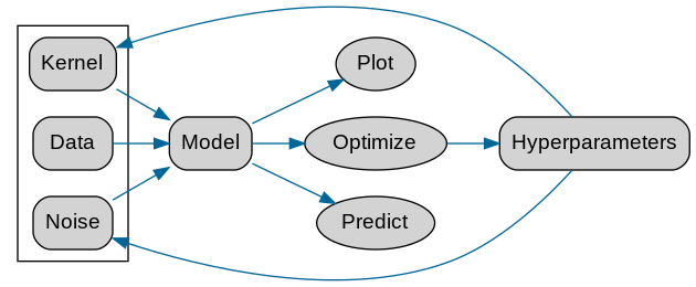
As for the data input, “Kernel” and “Noise” are input as parameters as in the previous article on Clojure, and GPy performs prediction and optimization for them.

The GPy web page includes tutorials using Jupyter. Some of them are transcribed below.
Basic Gaussian Process Regression Problem
As with GP in Clojure, specify kernel, create model, optimize and draw.
import GPy
import pandas as pd
import numpy as np
import matplotlib.pyplot as plt

kernel = GPy.kern.RBF(1)
# kernel = GPy.kern.RBF(1) + GPy.kern.Bias(1) + GPy.kern.Linear(1)


X = np.random.uniform(-3.,3.,(20,1))
Y = np.sin(X) + np.random.randn(20,1)*0.05
model = GPy.models.GPRegression(X, Y, kernel=kernel)
model.optimize()
model.plot()
plt.savefig('output/fig2.png')
Regression results when the kernel function is “kernel = GPy.kern.RBF(1) + GPy.kern.Bias(1) + GPy.kern.Linear(1)”, which represents complex kernel functions in terms of addition and subtraction.

The regression on 2-dimensional data is as follows. Matern is used here as kernel.
import GPy
import numpy as np
import matplotlib.pyplot as plt

kernel = GPy.kern.Matern52(2, ARD=True)

np.random.seed(seed=123)
N = 50
X = np.random.uniform(-3.,3.,(N, 2))
Y = np.sin(X[:,0:1]) * np.sin(X[:,1:2]) + np.random.randn(N,1)*0.05

model = GPy.models.GPRegression(X, Y, kernel)
model.optimize(messages=True, max_iters=1e5)
model.plot()
plt.savefig('output/fig3.png')

model.plot(fixed_inputs=[(0, -1.0)], plot_data=False)
plt.savefig('output/fig3-slice.png')
The regression curve for the case (slice) where some of the 2-dimensional inputs are fixed (1.0 for the input with index 0) is shown below.

Sparse Gaussian process regression
An approach called the auxiliary variable method, which treats some auxiliary variables (including input) of the data points of the Gaussian process as representative values of the input dimension to speed up the calculation.
import GPy
import pandas as pd
import numpy as np
import matplotlib.pyplot as plt

#Sample
np.random.seed(101)
N = 50
noise_var = 0.05

X = np.linspace(0,10,50)[:,None]
k = GPy.kern.RBF(1)
Y = np.random.multivariate_normal(np.zeros(N),k.K(X)+np.eye(N)*np.sqrt(noise_var)).reshape(-1,1)

kernel = GPy.kern.RBF(1)

m_full = GPy.models.GPRegression(X, Y, kernel=kernel)
m_full.optimize()

Z = np.hstack((np.linspace(-6, -3, 3), np.linspace(3, 6, 3)))[:,None]
# Z = np.linspace(-6, 6, 12)[:, None]
m_sparse = GPy.models.SparseGPRegression(X, Y, Z=Z)
m_sparse.optimize()
m_sparse.plot()
plt.savefig('output/fig4.png')
print(m_sparse.log_likelihood(), m_full.log_likelihood()) 
Bayesian GPLVM (latent variable model with Gaussian process)
The Gaussian Process Latent Variable Model calculates latent variables by assuming that each feature x is generated by a Gaussian process regression from the latent variable z. This method has the potential to extract features latent in the data better than direct principal component analysis from x. This method has the potential to extract features latent in the data rather than using direct principal component analysis from x.
For example, if we perform a principal component analysis on the OIL FLOW data in PRML using R, we obtain the following results.
library(R.matlab)
library(ggplot2)

d <- readMat('input/3Class.mat') #Download from the link in the text
N <- nrow(d$DataTrn)
K <- ncol(d$DataTrn)
D <- 2

## PCA
res_pca <- prcomp(d$DataTrn)
d_pca <- data.frame(X1=res_pca$x[ ,1], X2=res_pca$x[ ,2])
d_pca$class <- as.factor(apply(d$DataTrnLbls, 1, function(x) which(x == 1)))
p <- ggplot(data=d_pca, aes(x=X1, y=X2, color=class))
p <- p + geom_point(size=1.5, alpha=0.5)
ggsave(p, file='output/result-pca.png', dpi=300, w=5, h=4)
For this data, analysis with Bayesian GPLVM makes it possible to divide the data into potential finer classes.
from scipy.io import loadmat
import scipy.io as spio
import GPy
import matplotlib.pyplot as plt

d = spio.loadmat('input/3Class.mat')
X = d['DataTrn']
X -= X.mean(0)
L = d['DataTrnLbls'].nonzero()[1]
input_dim = 2 # How many latent dimensions to use

kernel = GPy.kern.RBF(input_dim, ARD=True) + GPy.kern.Bias(input_dim) + GPy.kern.Linear(input_dim) + GPy.kern.White(input_dim)
model = GPy.models.BayesianGPLVM(X, input_dim, kernel=kernel, num_inducing=30)
model.optimize(messages=True, max_iters=5e3)
model.plot_latent(labels=L)
plt.savefig('output/fig8.png')
The computation time takes only a few minutes. By the way, there is also an MCMC approach using R-Stan, but
library(R.matlab)
library(rstan)
library(ggplot2)

d <- readMat('input/3Class.mat')
N <- nrow(d$DataTrn)
K <- ncol(d$DataTrn)
D <- 2

## Bayesian GPLVM
data <- list(N=N, K=K, D=D, Y=t(scale(d$DataTrn, scale=FALSE)))
stanmodel <- stan_model(file='model/model.stan')
fit_vb <- vb(stanmodel, data=data, init=function(){ list(x=t(res_pca$x[,1:D])) },
	seed=123, eta=1, adapt_engaged=FALSE)
ms <- extract(fit_vb)
x_est <- t(apply(ms$x, c(2,3), median))
d_gplvm <- data.frame(x_est, class=d_pca$class)
p <- ggplot(data=d_gplvm, aes(x=X1, y=X2, color=class))
p <- p + geom_point(size=1.5, alpha=0.5)
ggsave(p, file='output/result-bgplvm.png', dpi=300, w=5, h=4)
Since this is an MCMC process, it will take several hours of processing time even if a high-performance machine is used. Other frameworks such as Stochastic Variational Inference for GP Regression and Parametric Nonparametric Gaussian Process Regression are also available.

コメント