Machine Learning Artificial Intelligence Digital Transformation Probabilistic Generative Models Deep Learning Nonparametric Bayesian and Gaussian processes Support Vector Machine Clojure Navigation of this blog
summary
Bayesian optimization is an applied technique that takes full advantage of the characteristics of Gaussian regression processes, which can make probabilistic predictions based on a small number of samples and a minimal number of processes.
What is Bayesian Optimization?
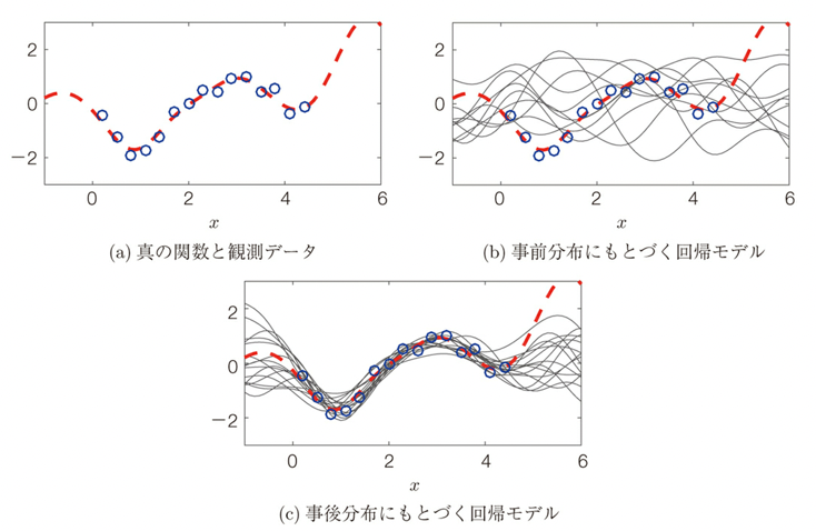
As described in the previous article “Gaussian Processes – The Advantages of Functional Clouds and Their Relationship to Regression Models, Kernel Methods, and Physical Models“, when a functional relationship between input x and output y (red dotted line) and some observed data (blue circles) are available, this functional relationship can be expressed as a Gaussian process as follows. process is expressed as follows, which represents the process of convergence of a random cloud-like distribution in the prior distribution when real data are given, and

Bayesian optimization, as described in “Spatial Statistics of Gaussian Processes, Application to Bayesian Optimization,” optimizes an acquisition function and an expected improvement function by combining the expected value and variance of the posterior probability obtained from the analysis of Gaussian processes (the optimization strategy is the Upper Confidence Bound (UCB) as described in “Overview of the Upper Confidence Bound (UCB) Algorithm and Examples of Implementation” strategy is used as the optimization strategy) to effect this convergence. In actual optimization, as shown in the figure below, the next measurement point is selected at which the prediction function of the Gaussian process generated from the real data has a large variance (and is calculated from the expected value) (the wide purple area in the figure below), the next prediction function is calculated reflecting the result, and then the prediction function is converged by selecting another point with a large variance (and is calculated from the expected value). The predictive function is then converged by selecting the point with more variance (and the expected value).

Similar to this approach, there is an existing method called experimental design. Like Bayesian optimization, experimental design uses discrete data and selects optimal parameters by focusing on variation (error), but the Bayesian optimization approach can be used for optimization by continuous values or variance/expected values, making it a more versatile approach.
For example, it can be used to sequentially extract the optimal combination of experimental parameters to be used next while conducting experiments in experimental design for medicine, chemistry, materials research, etc., to sequentially perform optimization while rotating the learning/evaluation cycle of hyper-parameters in machine learning, or to optimize functions by matching parts in the manufacturing industry. It is a technology that can be used in a wide range of applications, such as sequential optimization through a cycle of learning/evaluation of hyperparameters in machine learning, and optimization of functions by matching parts in manufacturing.
In python code, GPyOpt, a library based on GPy by the University of Sheffield, GPFlow and GPyTorch, which use Tensorflow and PyTorch, as well as GPyTorch, a library based on GPy, which was previously introduced in “GPy – A Framework for Gaussian Processes Using Python”. GPyTorch, or the Bayesian optimization function bayesopt implemented in MATLAB as part of the Stastics and Machine Learning Tollbox (paid service) are well-known examples.
In this article, we will discuss Bayesian optimization in Clojure using fastmath, a Clojure math library.
Implementation in Clojure
The implementation in Clojure was based on the Bayesian Optimization article by generateme, who has uploaded many statistical machine learning tools such as fastmath, cljplot, etc., and the fastmath library. Implementation of Gaussian Processes in Clojure” for an article on fastmath.
First, create a project file as usual with “lein new bo-test (arbitrary filename)”. prject.clj file should be as follows
(defproject bo-test2 "0.1.0-SNAPSHOT"
  :description "FIXME: write description"
  :url "http://example.com/FIXME"
  :license {:name "EPL-2.0 OR GPL-2.0-or-later WITH Classpath-exception-2.0"
            :url "https://www.eclipse.org/legal/epl-2.0/"}
  :dependencies [[org.clojure/clojure "1.10.1"]
                 [generateme/fastmath "1.4.0-SNAPSHOT"]
                 [cljplot "0.0.2-SNAPSHOT"]
                 [clojure2d "1.2.0-SNAPSHOT"] ]
  :repl-options {:init-ns bo-test2.core})
It should be noted here that although fastmath is now up to “2.1.8”, it is necessary to use “1.4.0-SNAPSHOT” as it is because the function definitions have changed significantly due to major changes in the SMILE 2.x API on which it is based.
The namespace of the file src/bo_test/core.clj and the library introduction part are as follows.
(ns bo-test2.core)

(require '[cljplot.build :as b]
         '[cljplot.core :refer :all]
         '[fastmath.core :as m]
         '[fastmath.kernel :as k]
         '[fastmath.random :as r]
         '[fastmath.optimization :as o]
         '[fastmath.classification :as cl]
         '[clojure2d.color :as c]
         '[clojure.java.io :as io]
         '[clojure.string :as str])
optimization
Let’s talk a little about optimization. The simplest form of optimization is to find the optimal value of a function (a black box function) in a non-analytic way, and Java and Pyhton mathematical libraries have various classes (functions) for such optimization.
As an example, consider the following complex black box function.
\[z=1+\left(\left(\frac{sin(2xy)}{xy}\right)+sin(x+y)+cos(y+y)+sin(2xy))\right)\]

In contrast, using BOBYQA, one of the optimization algorithms, and a wrapper for optimizer, one of the classes of fastmath, a Java math library, the optimization within a specific bounded region (bouns2) is shown below.
(defn black-box-function
  ^double [^double x ^double y]
  (+ 1.0 (* (m/sinc (+ 2.0 x y))
           (m/sin (+ x x))
           (m/cos (+ y y))
           (m/sin (* 2.0 x y)))))

(black-box-function -1.5 0.5)  ;; 1.0

(def bounds2 [[-1.0 0.5] [-2 -0.5]])

(o/maximize :bobyqa black-box-function2 {:bounds bounds2})  ;;[(-0.601666316911455 -1.4622938217249408) 1.8891426447312971]
In contrast, Bayesian optimization yields the following.
(def bo (o/bayesian-optimization black-box-function2 {:bounds bounds2}))

(first bo) ;; {:x [-0.5818284049054684 -1.7214731540148598], :y 1.6810441771166404,...

(select-keys (nth bo 25) [:x :y]) ;; {:x (-0.6014301541014717 -1.4624072382800395), :y 1.8891423521925965}


(def palette (reverse (:rdylbu-9 c/palette-presets)))
(def gradient (c/gradient palette))

(defn draw-2d
  [f bounds bayesian-optimizer iteration]
  (let [{:keys [util-fn gp xs]} (nth bayesian-optimizer iteration)
        cfg {:x (first bounds)
             :y (second bounds)
             :palette palette
             :contours 30
             :gradient gradient}]
  (xy-chart {:width 700 :height 700}
            (b/series [:contour-2d f (assoc cfg :position [0 1])]
                      [:scatter xs {:size 10
                                    :color (c/darken (first palette))
                                    :margins {:x [0 0] :y [0 0]}
                                    :position [0 1]
                                    :label "2d function with guessed points."}]
                      [:function-2d util-fn (assoc cfg :position [0 0]
                                                   :label "Utility function")]
                      [:contour-2d (fn [x y] (gp [x y]))
                       (assoc cfg :position [1 1]
                              :label "Gaussian processes - mean (interpolation)")]
                      [:contour-2d (fn [x y] (second (gp [x y] true)))
                       (assoc cfg :position [1 0]
                              :label "Gaussian processes - std dev")])
                  (b/add-axes :bottom)
                  (b/add-axes :left))))

(def draw-black-box2 (partial draw-2d black-box-function2 bounds2))

(save (draw-black-box2 bo 0) "results/black-box2.jpg")
Increasing the number of Bayesian optimization (bo) steps confirms convergence to the optimal value.

Here, the UCB as an optimization strategy is as follows.
(def bo (o/bayesian-optimization black-box-function2 {:bounds bounds2
                                                      :noise 0.01
                                                      :utility-function-type :ucb
                                                      :utility-param 0.1}))

(save (draw-black-box2 bo 15) "results/black-box2-ucb-low.jpg") 
The optimization strategy using ei is also shown below.
(def bo (o/bayesian-optimization black-box-function2 {:bounds bounds2
                                                      :noise 0.01
                                                      :utility-function-type :ei
                                                      :utility-param 0.01}))

(save (draw-black-box2 bo 15) "results/black-box2-ei-low.jpg")
Furthermore, the kernel function with Mattern is as follows.
(def bo (o/bayesian-optimization black-box-function2 {:bounds bounds2
                                                      :utility-function-type :ei
                                                      :kernel (k/kernel :mattern-12 2)
                                                      :noise 0.1}))

(save (draw-black-box2 bo 15) "/results/black-box2-wide.jpg")
There are many parameters that can be used in Bayesian optimization, and the convergence will differ depending on the optimization of these parameters.
The optimx package in R can be used to compare various optimizations.
library(optimx)

loglik <- function(x, param) {
  -sum(dnbinom(x, size = param[1], mu = param[2], log = TRUE))
}

set.seed(71)
data <- rnbinom(500, size = 10, mu = 5)
initparam <- c(10, 5)
optimx(par = initparam, fn = loglik, x = data, control = list(all.methods = TRUE))
                   p1       p2         value fevals gevals niter convcode kkt1 kkt2 xtimes
BFGS         9.889487 5.038007  1.190725e+03     14      5    NA        0   NA   NA   0.01
CG           9.892441 5.037995  1.190725e+03    305    101    NA        1   NA   NA   0.27
Nelder-Mead  9.892127 5.038049  1.190725e+03     41     NA    NA        0   NA   NA   0.02
L-BFGS-B     9.889511 5.038000  1.190725e+03     13     13    NA        0   NA   NA   0.03
nlm          9.889480 5.037999  1.190725e+03     NA     NA    11        0   NA   NA   0.01
nlminb       9.889512 5.038000  1.190725e+03      8     18     5        0   NA   NA   0.00
spg          9.889768 5.038000  1.190725e+03     24     NA    18        0   NA   NA   0.13
ucminf       9.889507 5.037997  1.190725e+03      9      9    NA        0   NA   NA   0.02
Rcgmin             NA       NA 8.988466e+307     NA     NA    NA     9999   NA   NA   0.00
Rvmmin             NA       NA 8.988466e+307     NA     NA    NA     9999   NA   NA   0.00
newuoa       9.889511 5.038000  1.190725e+03     34     NA    NA        0   NA   NA   0.02
bobyqa       9.889509 5.038000  1.190725e+03     27     NA    NA        0   NA   NA   0.01
nmkb         9.890341 5.037991  1.190725e+03     69     NA    NA        0   NA   NA   0.03
hjkb        10.000000 5.000000  1.190775e+03      1     NA     0     9999   NA   NA   0.02
Hyperparameter Search
Bayesian optimization can also be used to perform hyperparameter search, such as machine learning. As an example, the soar.csv file on kaggle (a dataset used by Gorman and Sejnowski in their study of sonar signal classification using neural networks. The file contains 111 patterns of sonar signals bounced off a metal cylinder at various angles, each pattern being a set of 60 values of energy in a certain frequency band ranging from 0.0 to 1.0 integrated over a certain time period. The label on each record contains the letter “R” if the object is a rock, while mines (metal cylinders) are labeled “M.”)
First, the data can be checked as follows.
(def dataset (with-open [data (io/reader "data/sonar.csv")]
               (mapv #(-> %
                          (str/trim)
                          (str/split #",")
                          (->> (map read-string))) (line-seq data))))

(count dataset) ;;208

(def xs (map butlast dataset))
(def ys (map (comp keyword last) dataset))

(frequencies ys)  ;;111
In contrast, the hyperparameter optimization in Ada boost is as follows
(defn ada-boost-params
  ^double [^double trees ^double nodes]
  (let [ada-boost (cl/ada-boost {:number-of-trees (int trees)
                                 :max-nodes (int nodes)} xs ys)]
    (:accuracy (cl/cv ada-boost))))

(def ada-bounds [[1 (count dataset)]
                 [2 (count dataset)]])

(ada-boost-params 10 20)

(def ada-boost-bo (o/bayesian-optimization ada-boost-params
                                           {:init-points 5
                                            :kernel (k/kernel :mattern-52 55.0)
                                            :noise 0.05
                                            :utility-param 0.1
                                            :bounds ada-bounds}))

(select-keys (first ada-boost-bo) [:x :y])

(defn draw-2d-2
  [bounds bayesian-optimizer iteration]
  (let [{:keys [gp xs]} (nth bayesian-optimizer iteration)
        cfg {:x (first bounds)
             :y (second bounds)
             :palette palette
             :contours 30}]
    (xy-chart {:width 700 :height 300}
              (b/series [:contour-2d (fn [x y] (gp [x y])) cfg]
                        [:contour-2d (fn [x y] (second (gp [x y] true)))
                         (assoc cfg :position [1 0]
                                :label "Gaussian processes - std dev")]
                        [:scatter xs {:size 10
                                      :color (c/darken (first palette))
                                      :margins {:x [0 0] :y [0 0]}
                                      :position [0 0]
                                      :label "Gaussian processes - mean (interpolation)"}])
              (b/add-axes :bottom)
              (b/add-axes :left))))

(save (draw-2d-2 ada-bounds ada-boost-bo 20) "results/ada-boost.jpg")
Next, hyperparameter optimization in SVM is performed.
(defn svm-params
  ^double [^double cp ^double cn]
  (let [cp (m/pow 10 cp)
        cn (m/pow 10 cn)
        svm (cl/svm {:c-or-cp cp :cn cn
                     :kernel (k/kernel :gaussian)} xs ys)]
    (m/log (:accuracy (cl/cv svm)))))

(def svm-bounds [[-6 6] [-6 6]])

(m/exp (svm-params 1 1))

(def svm-bo (o/bayesian-optimization svm-params
                                     {:init-points 5
                                      :kernel (k/kernel :mattern-52 1.5)
                                      :utility-param 0.3
                                      :noise 0.05
                                      :bounds svm-bounds}))

(m/exp (:y (nth svm-bo 10)))

(save (draw-2d-2 svm-bounds svm-bo 10) "results/svm.jpg")
We can confirm that the estimation of hyperparameters is more convergent in SVM compared to Ada-boost.

コメント