Evaluating Clustering
As introduced in the article “AI Algorithms for Business Use, Not Just Deep Learning,” k-means is one of the algorithms that should be applied first from the viewpoints of simplicity, versatility, data acquisition (training is possible even with a small amount of data), and readability. In this article, I would like to discuss evaluation techniques as a way to use k-means in a more advanced way. (From Clojure for Data Science)
Depending on the library, a k-mean evaluation will come out with the following evaluation results attached.
Inter-Cluster Density: 0.6135607681542804
Intra-Cluster Density: 0.6957348405534836
The ideal clustering is one in which the intra-cluster variance is small (or high) compared to the inter-cluster density.
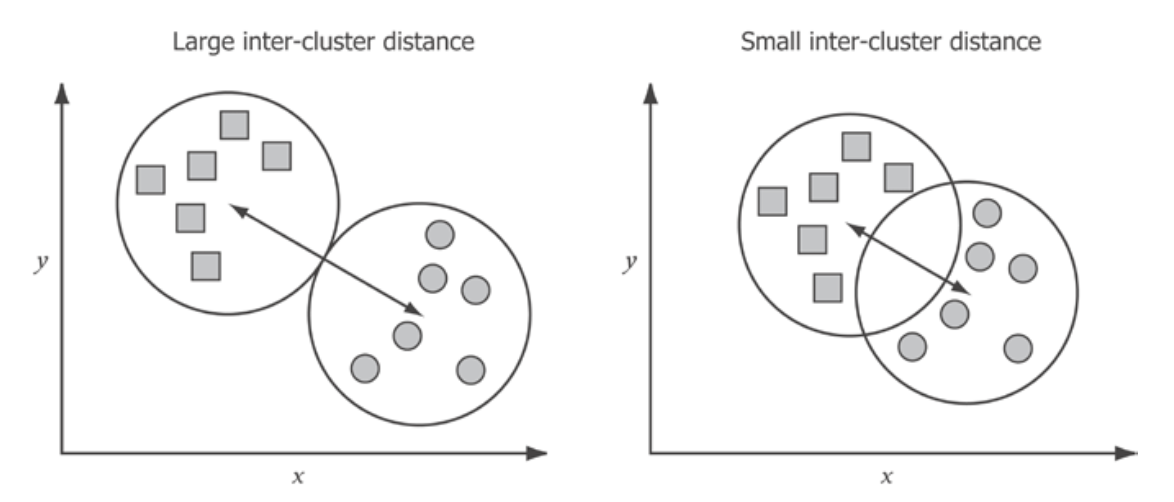
First, inter-cluster density is the average distance between cluster centers. Good clusters have centers that are never too close to each other. If they are, it means that clustering has created groups with similar characteristics and differentiated between cluster members that are difficult to support.

Intra-cluster density is an indicator of how compact the clusters are. Ideally, clustering identifies groups of items that are similar to each other. A compact cluster indicates that all items in the cluster are strongly similar.

Thus, the best clustering results will be those with high intra-cluster density and low inter-cluster density. However, it is not always clear how many clusters are justified by the data. The following figure shows the same data set grouped into various numbers of clusters, but it is difficult to say with certainty the ideal number of clusters.

The previous figure is intentional, but it illustrates a general problem with data clustering. In many cases, there is no clear “optimal” number of clusters, and the most effective clustering is highly dependent on the end use of the data.
However, by determining how the value of a given quality score varies with the number of clusters, one can infer which value is better. The quality score can be a statistic such as inter-cluster density or intra-cluster density. As the number of clusters approaches the ideal, the value of this quality score is expected to improve. Conversely, as the number of clusters deviates from the ideal, a decrease in quality is expected. Therefore, in order to know the adequacy of the number of clusters in the data set, it is necessary to run the algorithm many times with different values of k.
squared error
One of the most common measures of cluster quality is the sum of squared errors (SSE). For each point, the error is the measured distance to the nearest cluster centroid. Thus, the sum of the clustering SSE is the sum over all clusters from the clustered point to its corresponding centroid. (RSME((Root Mean Squared Error))
\[RMSE=\sqrt{\frac{1}{n}\displaystyle\sum_{i=1}^k\sum_{x\in S}||\mathbf{x}-\mu_i||^2}\]
Here, μi is the central value (average) of cluster Si, k is the total number of clusters, and n is the total number of points.
When RMSE is plotted against the number of clusters, it decreases as the number of clusters increases. The RMSE error (variance from the mean of the original data set) is largest when there is only one cluster, while the RMSE is smallest when all points are within their own cluster (zero RMSE). These extremes obviously do not explain the structure of the data well. However, RMSE does not decrease in a straight line. It decreases rapidly as the number of clusters is increased from one and decreases slowly as the “natural” number of clusters is exceeded.
Therefore, one way to determine the ideal number of clusters is to plot how RMSE varies with respect to the number of clusters. This is called the elbow method.
Estimating the optimal k-value using the elbow method
To determine the value of k using the elbow method, k-means must be rerun many times. The following example will be calculated for all k from 2 to 21.

The above graph shows that the rate of change in RMSE slows down when k exceeds about 13 clusters and becomes less as the number of clusters is further increased. Thus, the graph indicates that about 13 clusters is appropriate.
Although the elbow method provides an intuitive way to determine the ideal number of clusters, it may be difficult to apply in practice, because when k is small or when there is a lot of noise in the RMSE, it may not be clear where the elbow is located or whether an elbow exists.
Since clustering is an unsupervised learning algorithm, we assume here that the internal structure of the clusters is the only way to verify the quality of the clustering. If the true cluster labels are known, then external verification measures (such as entropy) can be used to validate the success of the model.
We discuss two other clustering evaluation schemes, the Dunn index and the Davies-Bouldin index. Both are internal evaluation schemes, meaning that they only look at the structure of the clustered data. Each aims to identify the clustering that produced the most compact and well-separated clusters, and does so in different ways.
Estimation of optimal k-value by Dunn Index
The Dunn Index provides another way to select the optimal number of k. The Dunn Index does not consider the average error remaining in the clustered data, but rather the ratio of the two “worst case” cases (minimum distance between the two cluster centers, divided by the maximum cluster diameter). In general, we want the inter-cluster distance to be large and the intra-cluster distance to be small, so a higher value for this index indicates better clustering.
For k clusters, the Dunn index can be expressed as follows.
\[DI_m=\frac{\min_{1≤i<j≤k}\delta(C_i,C_j)}{\max_{1≤m≤k}S_m}\]
where δ(Ci,Cj) is the distance between two clusters Ci and Cj, max1≤m≤k Sm is the size (or scatter) of the largest cluster.
There are several possible ways to compute the scatter of clusters. One can take the distance between the two farthest points in a cluster, the average of all pairwise distances between data points in a cluster, or the average of each data point from the cluster center value itself.
Using the dunn-index function, a scatterplot of clusters from k=2 to k=20 can be created as follows.

A higher Dunn index indicates better clustering. Thus, the best clustering is k=2, followed by k=6, and then k=12 and k=13.
Estimation of optimal k-value by Davies-Bouldin index
The Davies-Bouldin index is an alternative evaluation scheme that measures the average of the ratio of size to separation for all values in a cluster. It finds, for each cluster, the alternative cluster with the largest ratio of total cluster size divided by distance between clusters; the Davies-Bouldin index is defined as this value averaged over all clusters in the data.
\begin{eqnarray}D_i&=&\max_{i≠j}\frac{S_i+S_j}{\delta(C_i,C_j)}\\DB&=&\frac{1}{n}\displaystyle\sum_{i=1}^n D_i\end{eqnarray}
where δ(Ci,Cj) is the distance between the two cluster centers Ci and Cj, and Si and Sj are the scatter. Here is an example of Davies-Bouldin for clusters k=2 to k=20 plotted on a scatter plot.

Unlike the Dunn index, the Davies-Bouldin index is an excellent clustering scheme that looks for clusters with compact size and long inter-cluster distance. The above results show that k=2 is the ideal cluster size, followed by k=13.
On the optimization of K-means
k-means is one of the most popular clustering algorithms because of its relatively easy implementation and its ability to cope well with very large data sets. Despite its popularity, however, it has several drawbacks.
One of the drawbacks is that k-means is stochastic and is not guaranteed to find a globally optimal solution for clustering. In fact, the algorithm is very sensitive to outliers and noisy data, and the quality of the final clustering can be highly dependent on the location of the initial cluster center point. This can be rephrased to say that k-means regularly finds local rather than global minima.
Mahalanobis distance
Given a data set of red points, consider whether the blue or green point is farther away from the data set. Considering the Euclidean distance from the mean of the data group (point X), the green and blue points are approximately the same distance. However, a more natural interpretation is to consider the green point to be farther away from the data group.

This suggests that when considering the distance from a group of data, it is necessary to have an index that considers not only the simple distance, but also the scattering of the data in various directions. The Mahalanobis distance is what makes this possible. The definition of the Mahalanobis distance is as follows: If the mean vector (vec{mu}) of a group of data and the variance-covariance matrix is Σ, the Mahalanobis distance of a vector (vec{x}) can be expressed as follows.
\[d_{Mahalanobis}=\sqrt{(\vec{x}-\vec{\mu})^T\Sigma^{-1}(\vec{x}-\vec{\mu})}\]
By measuring the Mahalanobis distance of each variable, it is possible to determine points that are obviously far from the cluster (anomalous points).
As an example, given the following data (arrows indicate anomalous points)

If we measure the Euclidean distance for each variable, we get the following, with no difference between any of the points.

When plotted in terms of Mahalanobis distance, the following can be seen, confirming that only one point deviates significantly.

If the data are one-dimensional, the mean vector is a scalar μ and the variance-covariance matrix is also a scalar σ2. Thus, the Mahalanobis distance is as follows.
\[d=\sqrt{(x-\mu)\cdot\frac{1}{\sigma^2}\cdot (x-\mu)}=\frac{|x-\mu|}{\sigma}\]
This will be the difference from the mean normalized by the standard deviation σ, and \(\frac{x-\mu}{\sigma}\) with the absolute value removed will be what is known as the z-score.
Curse of the dimension
The challenge that the Mahalanobis distance measure cannot overcome is known as the “curse of dimensionality”. This refers to “the tendency for all points to become equally distant from other points as the dimensionality of the data set is increased. For example, the following figure shows the difference between the minimum and maximum distance in a composite generated data set of 100 points. As the number of dimensions approaches the elements of the set, the minimum and maximum distances for each pair of elements become closer together, so that in a 100-dimensional, 100-point data set, every point is equally far from every other point.

For more information on k-means in python, please refer to “Overview of k-means, its applications, and implementation examples“.

コメント