Machine Learning Artificial Intelligence Digital Transformation Probabilistic Generative Models Deep Learning Nonparametric Bayesian and Gaussian processes Support Vector Machine Clojure Navigation of this blog
Probabilistic Programming with Clojure
Stan, BUSGS, etc., which were previously discussed in probabilistic generative models such as Bayesian models, are also called Probabilistic Programming (PP). PP is a programming paradigm in which probabilistic models are specified in some form and inference on those models is automatically performed. Their purpose is to integrate probabilistic modeling and general-purpose programming to build systems combined with various AI techniques for a variety of uncertain information, such as stock price prediction, movie recommendations, computer diagnostics, cyber intrusion detection, and image detection.
The programming language used for probabilistic programming is called Probabilistic Programming Language (PPL), which is implemented in R. Stan, BUGS, Julia’s library Picture, Turing, and Gen, PyStan, PyMC, pomegranater, Lea, and bayesloop as libraries in python, Edward as a library in TensorFlow, Tensorflow Probability, Pyro in PyTorch, BLOG in Java, Dyna and ProbLog in Prolog, Church in Schema, Anglican in Clojure, Distributions, and many others have been proposed.
For reference information, see “The Design and Implementation of Probabilistic Programming Languages,” “Towards common-sense reasoning via conditional simulation: Towards common-sense reasoning via conditional simulation: legacies of Turing in Artificial Intelligence,” “Practical Probabilistic Programming,” and “Probabilistic-Programming.org,” among others.
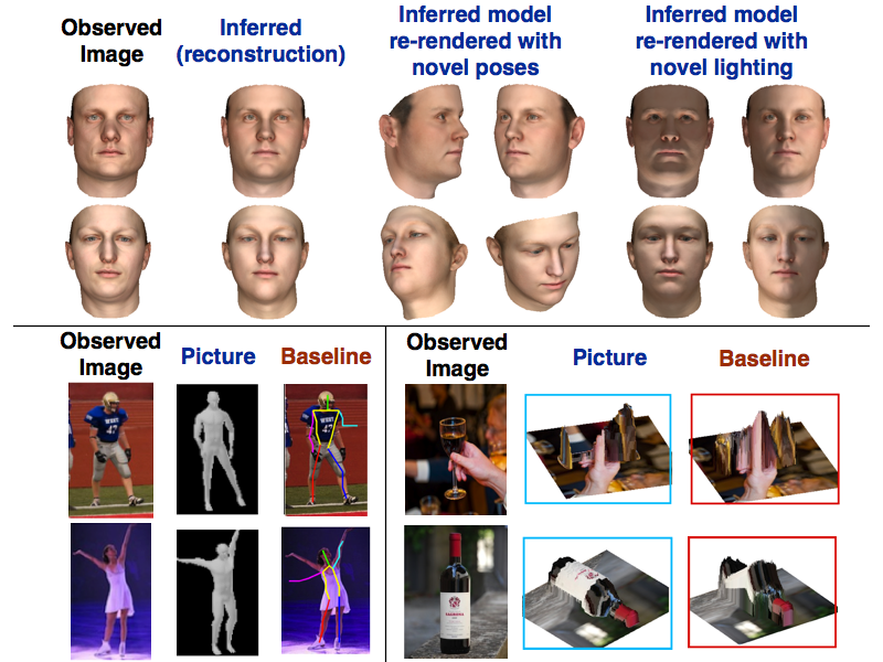
Recent examples of his research include the aforementioned probabilistic generative model using Julia’s Picture to generate 3D image backing from 2D images and extract feature data.

Application to Reinforcement Learning

Application to meta-reasoning

Application to constrained stochastic simulation.

Probabilistic programming has been applied in various fields, such as the following.
In this article, we will discuss the Clojure approach to probabilistic programming, including Anglican and Distributions, etc. In this article, we will discuss Anglican, which is based on Schema’s Church.
Anglican is defined as follows in the official website. Anglican is a probabilistic programming language integrated with Clojure and ClojureScript.
Anglican incorporates a sophisticated theoretical background that you are invited to explore, but its value proposition is to enable intuitive modeling in a probabilistic environment. It is not an academic exercise, but a practical everyday machine learning tool that makes probabilistic reasoning effective.
Do you interact with users or remote systems? Then you often have the unfortunate experience of their unexpected behavior. Mathematically speaking, we observe non-deterministic or probabilistic behavior, and Anglican allows us to represent the random variables that capture all this probability theory, allowing us to learn from the data and make informed decisions in our Clojure programs.”
For details, please refer to the official website and the paper “A New Approach to Probabilistic Programming Inference“.
The following is a description of the specific implementation. First, Gorilla Repl is introduced as a PF for evaluation.

Gorilla Repl is a web-based development environment equivalent to Python’s Jupyter notebook (recently, it seems that Jupyter can be used directly, but we will spare you the explanation of that).
> lein new app gr-test(Any project name)It is important to note that this is an application project template, not the simple project template creation we have been using. After that, write the Grilla Repl plugin in the project.clj file of the project created above.
(defproject gr-test "0.1.0-SNAPSHOT"
  :description "FIXME: write description"
  :url "http://example.com/FIXME"
  :license {:name "EPL-2.0 OR GPL-2.0-or-later WITH Classpath-exception-2.0"
            :url "https://www.eclipse.org/legal/epl-2.0/"}
  :dependencies [[org.clojure/clojure "1.11.1"]]
  :main ^:skip-aot gr-test.core
  :target-path "target/%s"
  :plugins [[org.clojars.benfb/lein-gorilla "0.6.0"]]
  :profiles {:uberjar {:aot :all
                       :jvm-opts ["-Dclojure.compiler.direct-linking=true"]}})
The official website says to put “[lein-gorilla “0.4.0”]”, but if you put that, it will not work. Instead, you need to insert [org.clojars.benfb/lein-gorilla “0.6.0”] as shown above.
From the top of the project directory, type “lein gorilla” in the terminal to launch gorilla-repl as shown below.
>lein gorilla
………………………………………
Gorilla-REPL: 0.6.0
Unable to reach update server.
Started nREPL server on port 49989
Running at http://127.0.0.1:49991/worksheet.html .
Ctrl+C to exit.
If you access “http://127.0.0.1:49991(the address changes each time the server is launched)/worksheet.html” with any browser, a web REPL environment like the one shown above will be launched. The command HELP is displayed by pressing “CTRL” + g (twice quickly), but basically, as with Jupyter, you can write code and evaluate it by pressing “shift” + “enter”.
Next, we will discuss the use of anglican. anglican example can be downloaded from problog/anglican example in git, and the workshhets file in it can be copied to the project folder (gr-test) that you have just created. Copy the file to the project folder you just created (gr-test), and use the gorilla REPL by pressing “CTRL” + g (twice quickly) and selecting “Load a worksheet”.
First, set the necessary libraries in the project.clj file of the project (gr-test) you just created.
(defproject gr-anglican "0.1.0-SNAPSHOT"
  :description "FIXME: write description"
  :url "http://example.com/FIXME"
  :license {:name "EPL-2.0 OR GPL-2.0-or-later WITH Classpath-exception-2.0"
            :url "https://www.eclipse.org/legal/epl-2.0/"}
  :dependencies [[org.clojure/clojure "1.11.1"]
                 [anglican "1.1.0"]
                 [net.mikera/core.matrix "0.62.0"]]
  :main ^:skip-aot gr-anglican.core
  :target-path "target/%s"
  :plugins [[org.clojars.benfb/lein-gorilla "0.6.0"]]
  :profiles {:uberjar {:aot :all
                       :jvm-opts ["-Dclojure.compiler.direct-linking=true"]}})
Now consider a classification problem based on the following equation.
\[p(x,c|\theta)=p(x|c,\theta)p(c|\theta)=N(x|\mu_c,\Sigma_c)\pi_c\]
c∈0,…,C is the class of classification, x∈ℝD is the set of features, and θ is the parameter set of the classification, which consists of the prior probability π, the mean μc and the variance Σc. When the classification of each data point is known (i.e., when a dataset is available), generally referred to as a classification task, this model can be called the classification model. This model is called multiclass Gaussian discriminant analysis (GDA). If the correct classification of each data point is not known, but only a list of observed features, this model is called a Gaussian Mixture Model (GMM).
Here we consider an approach that can consider both labeled and unlabeled data points.
We first define the following GDA function using Anglican’s log-sum-exp function.
(defdist gda [pi feature-dists]

  [class-dist (discrete pi)
   C (count pi)]

  (sample* [this]
           (let [my-class (sample* class-dist)
                 my-features (sample* (nth feature-dists my-class))]
             [my-class my-features]))

  (observe* [this [my-features my-class]]
            (if (not (nil? my-class))
              (+
                (observe* class-dist my-class)
                (observe* (nth feature-dists my-class) my-features))

              (reduce log-sum-exp
                      (map

                        #(+'
                           (observe* class-dist %)
                           (observe* (nth feature-dists %) my-features))

                        (range C))))))
The following functions are used to classify individual data points using the above model: the classification-log-probabilities function takes a GDA instance and a specific set of features, and returns this class-specific set of features as a list of non-normalized log probabilities. The classification-probabilities function calls the above function, exponentiates and normalizes the result, and returns the normal probabilities.
If a predicted classification result, rather than a distribution over the classifications, is needed, the classify-feature function is used. This would compute the likelihood of each classification using log probabilities and simply return the most probable classification among them using the index-of-maximum function.
(defn classification-log-probabilities [gda-dist feature]
  (map
    (fn [c] (observe* gda-dist [feature c]))
    (range (:C gda-dist))))

(defn classification-probabilities [gda-dist feature]
  (let [unnormalized (classification-log-probabilities gda-dist feature)
        sum (reduce log-sum-exp unnormalized)
        normalized (map #(- % sum) unnormalized)]
    (map #(Math/exp %) normalized)))


(defn index-of-maximum [lst]
  (second
    (apply max-key first
           (map
             (fn [x y] [x y])
             lst
             (range)))))

(defn classify-feature [gda-dist feature]
  (let [unnormalized (classification-log-probabilities gda-dist feature)]
    (index-of-maximum unnormalized)))
The following simple example confirms the above. It shows how to create a GDA distribution with a specified feature distribution and prior classification probability using the above GDA distribution and helper functions. Then, using that GDA, the feature set
is classified and the probability of each classification is calculated.
(def feature-dist-1 (mvn [0 0] [[4 3] [3 4]]))
(def feature-dist-2 (mvn [0 10] [[10 -3] [-3 5]]))
(def feature-dist-3 (mvn [10 10] [[6 0] [0 8]]))

(def pi [1 1 1])

(def my-gda (gda pi (list feature-dist-1 feature-dist-2 feature-dist-3))) ;;training data

(def x [5 5]) ;; test data

(def probs (map #(Math/round (* 100 %)) (classification-probabilities my-gda x)))

(plot/bar-chart '(0 1 2) probs)
(reduce str (map #(str (Math/round (* 100 %)) "% ") (classification-probabilities my-gda x)))
;; "43% 41% 15% "
(str "The feature " x " has classification " (classify-feature my-gda x))
;;The feature [5 5] has classification 0"
The above only works if the correct classification probability pi and the correct feature distribution for each classification are known. The code below does this by placing prior distributions on these parameters, inferring them from the given data, and outputting the posterior predictions for the classification of data point x.
;; HYPERPARAMETERS (for priors):

(def nu [1 1 1])
(def alpha [1 1])


;; PRIORS:

(def mu-priors (mvn nu (mat/identity-matrix 3)))
(def sigma (mat/identity-matrix 3))
(def pi-prior (dirichlet alpha))


(defquery gda-trainer [data x]
  (declare :primitive mat/zero-matrix mat/to-vector mat/identity-matrix gda classification-probabilities)
  (let [N (count data)

        ;; sample parameters

        mu1 (sample mu-priors)
        mu2 (sample mu-priors)
        pi (sample pi-prior)

        ;; construct GDA distribution

        feature-dists (list (mvn mu1 sigma) (mvn mu2 sigma))
        gda-dist (gda pi feature-dists)]


    ;; condition on data
    (loop [n 0]
      (if (< n N)
        (do
          (observe gda-dist (nth data n))
          (recur (+ n 1)))))

    ;; now project the type of x
    (classification-probabilities gda-dist x)))
As an example, the parameters of the GDA distribution are inferred from the following data. It should be noted that in this data, some features have known classifications. However, some features have unknown classifications, so in order to learn the parameters, the probabilistic program must sum over all possible classifications. In particular, we note that no classification is known to be type 0.
Given this data, we do approximate the a posteriori classification of the feature set x.
(def dataset [
               [[3 3 3] 1]
               [[1 1 1]]
               [[0 0 0]]
               [[5 5 5] 1]
               [[4 4 4] 1]
               [[-1 -1 -1]]
               [[-2 0 0]]

               ])

(def x [1.5 1 1])
Actually learning the parameters of this type of classification problem is a rather complex inference problem. Here we use Anglican’s IPMCMC inference algorithm and 100,000 simulations to approximate the true posterior distribution.
(def S 100000)
(def particles 100)
(def nodes 10)

(def samples (take S (drop S
                           (doquery :ipmcmc gda-trainer [dataset x]
                                    :number-of-particles particles :number-of-nodes nodes))))

(def weights (map :log-weight samples))
(def projections (map :result samples))

(take-last 10 projections)

;;((0.538848314823797 0.46115168517620253) (0.538848314823797 0.46115168517620253)
   (0.538848314823797 0.46115168517620253) (0.538848314823797 0.46115168517620253)
   (0.538848314823797 0.46115168517620253) (0.9837451961913958 0.016254803808604182)
   (0.9837451961913958 0.016254803808604182) (0.9837451961913958 0.016254803808604182)
   (0.9837451961913958 0.016254803808604182) (0.9837451961913958 0.016254803808604182))
The final results can be summarized as follows
(defn calculate-mean [series]
  (empirical-mean
    (partition 2
               (interleave series weights))))

;; this will work better
(def percentages (map #(Math/round (* 100 %)) (calculate-mean projections)))

(plot/bar-chart (range (count percentages)) percentages)

(reduce str (map #(str % "% ") percentages))
;;"89% 11%"
It is obtained with 89% likelihood that data point X is not in Classification 1 but in Classification 0.

コメント