Machine Learning Artificial Intelligence Digital Transformation Probabilistic Generative Models Deep Learning Nonparametric Bayesian and Gaussian processes Support Vector Machine Clojure Navigation of this blog
Chinese resturant process (CRP) using Clojure and its application to mixed Gaussian distributions
From Anglican example. The CRP (Chinese resturant process), previously described in “Estimating the Number of Topics in a Topic Model – Dirichlet Process, Chinese Restaurant Process, and Stick Folding Process“, is a stochastic process that describes a particular data generating process. Mathematically, this data generating process is one that, at each step, samples a new integer from the set of possible integers, with a probability proportional to the number of times that particular integer has been sampled so far, with a constant probability of sampling a new integer that has not been seen before. It shall be.
So, intuitively, this process is (naturally) explained by the metaphor of a customer entering a Chinese restaurant.
This Chinese restaurant has an infinite number of tables, and at 12:00 there are no customers; at 12:01 a customer enters the restaurant and is seated at table 1. At this time, the state of the CRP is simply (1): one customer is seated at one table; at 12:02 another customer enters the restaurant, buys a dish, and tries to take a seat. However, this customer must choose whether to sit at table 1 with the previous customer or at the newly vacant table 2. This process goes on and on. At each point in time, the probability that a customer chooses a new table is a function of the parameter α in the CRP and the number of people sitting at each table. Customers are drawn to the table at which more customers are seated.
This Chinese restaurant process has been put to practical use as part of a model for an infinite parameter classification task. Suppose we have in front of us a row of N individuals that we want to classify into groups based on some attribute. If the number of groups present is known, this problem can be easily solved. Basically, we can find the individuals that are most similar to each other and infer the average characteristics of each group. However, if the number of groups is not known in advance, this problem is not as simple. This is because there is no obvious upper limit to the number of groups in the true population, and one may have to propose an infinitely large number of groups to solve this problem.
This would be the problem that the CRP seeks to solve. Intuitively, each individual is assigned to a “table” representing its classification. When faced with a new individual, the probability that the individual will be assigned to an existing classification depends on how common that classification was, and to some extent on the probability that the individual will be assigned to an entirely new classification.
With respect to this CRP, we describe an approach using anglican, the probabilistic programming framework of Clojure introduced in the previous article. Gorilla Repl is used as the implementation environment. As before, create a new project file with “lein new app (gr-anglican;project folder name)” and set the project.clj file in the created project folder as follows.
(defproject gr-anglican "0.1.0-SNAPSHOT"
  :description "FIXME: write description"
  :url "http://example.com/FIXME"
  :license {:name "EPL-2.0 OR GPL-2.0-or-later WITH Classpath-exception-2.0"
            :url "https://www.eclipse.org/legal/epl-2.0/"}
  :dependencies [[org.clojure/clojure "1.11.1"]
                 [anglican "1.1.0"]
                 [org.clojure/data.csv "1.0.1"]
                 [net.mikera/core.matrix "0.62.0"]
                 ;[plotly-clj "0.1.1"]
                 ;[org.nfrac/cljbox2d "0.5.0"]
                 ;[quil "3.1.0"]
                 ]
  :main ^:skip-aot gr-anglican.core
  :target-path "target/%s"
  :plugins [[org.clojars.benfb/lein-gorilla "0.6.0"]]
  :profiles {:uberjar {:aot :all
                       :jvm-opts ["-Dclojure.compiler.direct-linking=true"]}})
In this article, we focus on estimating the hyperparameter of the CRP, the number α. α is a pseudo number, which can be interpreted approximately as the likelihood of assigning a new individual to a new group rather than an existing group. Importantly, a given value of α may or may not be suitable for modeling a given data set. For example, if faced with a data set in which all individuals belong to the same group (1 1 1 1 1 1 1), a high value of α would be inappropriate because the probability of each individual going to a new group (new table) would be low. On the other hand, for a data set like (0 1 2 3 4 5 6 7 8 9), a high value of α would be highly appropriate.
In a Bayesian setting, one would place a prior distribution on the value of α, calculate the posterior distribution of the value of α given the true data, and use this posterior distribution to return a prediction of the next individual’s classification.
First, the namespace settings are as follows.
(ns gr-anglican
  (:require [gorilla-plot.core :as plot]
            [clojure.core.matrix :as m])
  (:use clojure.repl
        clojure.pprint
        [anglican core runtime emit stat]))
The next step is to define the model (function) of the random process and crp.
(defprotocol random-process2
  (evidence [this]
            "returns the log model evidence of the current state of the process"))


(defn crp-evidence [counts alpha]
  (let [N (reduce + (vals counts)) ;; this is the total # of customers, of samples seen
        C (count counts)] ;; this is the # of tables used so far
    (+
      (* C (Math/log alpha))
      (reduce + (map log-gamma-fn (vals counts))) ;; log-gamma-fn is factorial shifted by 1
      (log-gamma-fn alpha)
      (- (log-gamma-fn (+ alpha N))))))

(defproc CRP-new
  [alpha] [counts {}]
  (produce [this] (categorical-crp counts alpha))
  (absorb [this sample]
          (CRP-new alpha (update-in counts [sample] (fnil inc 0))))

  random-process2
  (evidence [this]
            (crp-evidence counts alpha)))
The estimation of CRP here is as follows.
;; train CRPs on some samples and return the predictions:
(defquery predict [samples alpha]
  (declare :primitive CRP-new evidence)
  (let [crp (loop [n 0
                   crp (CRP-new alpha)]
              (if (= n (count samples))
                 crp
                 (recur (+ n 1)
                        (absorb crp (nth samples n)))))]
    {:sample (sample (produce crp)), :evidence (evidence crp)}))

;; here are the samples we'll use:
(def samples '(0 1 1 1 1 2 2 3 3 3 3 1 1 2 2 3 3 3 3 4 4 5 5 6 6 6 6 6 6 7 7 8))
It is not immediately clear what alpha value would best summarize the above data. Customers do not overwhelmingly sit at the same table, but there is a noticeable tendency to prefer the table where they are already sitting. To get an idea of the impact of the parameter α, we compare the predictions of the CRP model for different values of α.
(def S 10000)
(def results-1 (map :sample (map :result (take S (doquery :importance predict [samples 0.1])))))
(def results-2 (map :sample (map :result (take S (doquery :importance predict [samples 5])))))
(def results-3 (map :sample (map :result (take S (doquery :importance predict [samples 50])))))
(plot/compose
(plot/histogram results-1 :normalize :probability :bins 10 :plot-range [[0 10] [0 1]] :color "blue")
(plot/histogram results-2 :normalize :probability :bins 10 :plot-range [[0 10] [0 1]] :color "green")
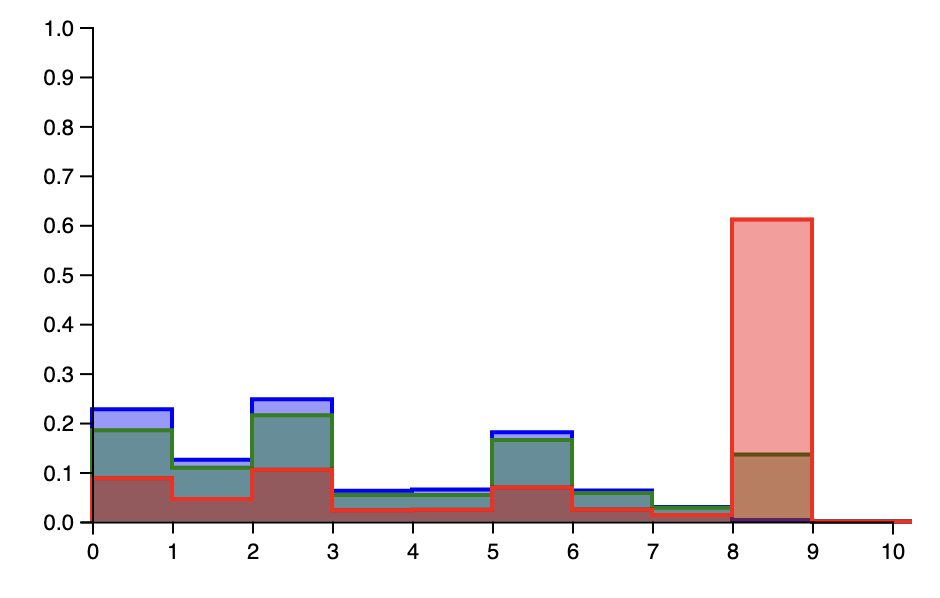
(plot/histogram results-3 :normalize :probability :bins 10 :plot-range [[0 10] [0 1]] :color "red"))The graphs output from these show that there are marked differences among the three models.

The blue model (α = 0.1) is in some ways the most “conservative” model. For a new customer, it is extremely likely to predict that the customer will join an already established table. In contrast, the red model (α = 50) is more “adventurous.” It is overwhelmingly likely to predict that a customer will join a new table that has not yet been settled. The Green model assigns a medium probability to each of these outcomes, making it a model that is also clearly, but not overwhelmingly, biased toward existing tables.
However, it is true that some of these CRPs are better than others at predicting our particular data set. Below is a code that plots the log confidence of the CRP models for a range of hyperparameter α.
(def alphas [0.01 0.05 0.1 0.5 1 5 10 50 100])

(defn find-evidence [alpha]
  (:evidence (:result (first (doquery :importance predict [samples alpha])))))

(def evidences (map find-evidence alphas))

(plot/list-plot (map (fn [a e] [(/ (Math/log a) (Math/log 10)) e])
                     alphas evidences))
The following is a graph of the output.

The optimal CRP appears to be an alpha between approximately 0.1 and 20 (the x-axis in the above graph is on a logarithmic scale, with 10 as the reference). Here, we deduce the correct value of alpha by taking a uniform prior distribution between 0 and 20.
(def alpha-prior (uniform-continuous 0 20))

(defquery predict [samples]
  (declare :primitive CRP-new)
  (declare :primitive evidence)
  (let [alpha (sample alpha-prior)
        crp (loop [n 0
                   crp (CRP-new alpha)]
              (if (= n (count samples))
                crp
                (recur (+ n 1)
                       (absorb crp (nth samples n)))))]
    (observe (flip (exp (evidence crp))) true)
    {:sample (sample (produce crp)), :alpha alpha}))
(def S 25000)

(def results (take S (map :result (doquery :smc predict [samples] :number-of-particles S))))
(def projections (map :sample results))
(def alphas (map :alpha results))

(plot/compose
  (plot/histogram (repeatedly S #(sample* alpha-prior)) :normalize :probability :color "green" :plot-range [[0 20] [0 0.3]])
  (plot/histogram alphas :normalize :probability))

(plot/histogram projections :normalize :probability :bins 10 :plot-range [[0 10] [0 1]])
The figure below shows a comparison of the prior distribution for the parameter α and the posterior distribution for the parameter α.

This result confirms that the correct value of α is approximately 5. However, the posterior prediction is a skewed distribution and does not completely rule out higher alpha values such as 14 or 15. However, lower alpha values are highly excluded.
Furthermore, the following figure shows the results of the posterior predictive distribution for the next output of the CRP.

Since we conclude that the value of α is likely to be moderate relative to the number of data sets, our posterior predicts that the probability of a customer sitting at a new table is moderate. (see green distribution above).
We can consider a Gaussian mixture model with this CRP.
(ns gr-anglican
  (:require [gorilla-plot.core :as plot]
            [clojure.core.matrix :as m]
            [anglican.stat :as s]
            :reload)
  (:use clojure.repl
        [anglican
          core runtime emit
          [state :only [get-predicts get-log-weight]]
          [inference :only [collect-by]]]))

(defn kl-categorical
  "KL divergence between two categorical distributions"
  [p-categories q-categories]
  (let [p-norm (reduce + (map second p-categories))
        q-norm (reduce + (map second q-categories))
        q (into {} (for [[c w] q-categories]
                     [c (/ w q-norm)]))]
    (reduce +
            (for [[c w] p-categories]
                   (if (> w 0.0)
                     (* (/ w p-norm)
                        (log (/ (double (/ w p-norm))
                                (double (get q c 0.0)))))
                     0.0)))))
Set up a model for CRP.
(defquery crp-mixture
  "CRP gaussian mixture model"
  [observations alpha mu beta a b]
  (let [precision-prior (gamma a b)]
    (loop [observations observations
           state-proc (CRP alpha)
           obs-dists {}
           states []]
      (if (empty? observations)
          (count obs-dists)
        (let [state (sample (produce state-proc))
              obs-dist (get obs-dists
                            state
                            (let [l (sample precision-prior)
                                  s (sqrt (/ (* beta l)))
                                  m (sample (normal mu s))]
                              (normal m (sqrt (/ l)))))]
          ;(observe obs-dist (first observations))
          (recur (rest observations)
                 (absorb state-proc state)
                 (assoc obs-dists state obs-dist)
                 (conj states state)))))))
Predictions are made for the following dummy data
(def data
  "observation sequence length 10"
  [10 11 12 -100 -150 -200 0.001 0.01 0.005 0.0])

(def posterior
  "posterior on number of states, calculated by enumeration"
  (zipmap
    (range 1 11)
    (mapv exp
        [-11.4681 -1.0437 -0.9126 -1.6553 -3.0348
         -4.9985 -7.5829 -10.9459 -15.6461 -21.6521])))
Make a prediction and plot the results.
(def number-of-particles 100)
(def number-of-samples 50000)

(def samples
  (->> (doquery :lmh crp-mixture
                [data 1.72 0.0 100.0 1.0 10.0]
                :number-of-particles number-of-particles)
       (take number-of-samples)
       doall
       time))

(plot/bar-chart (sort (keys posterior))
                (map #(get empirical-posterior % 0.0)
                     (sort (keys posterior))))
The forecast results from the mixed Gaussian model combined with CRP are shown in the figure below.

Very close to the distribution of the correct data is predicted.
(let [p (into (sorted-map) posterior)]
	(plot/bar-chart (keys p)
    	            (vals p)))

コメント