State Space Model with Clojure: Implementation of Kalman Filter
The state-space model described in “Time Series Data Analysis (1) State Space Model” was mainly used as a tool for analyzing changes on a time axis, but in fact, as described in “Difference between Hidden Markov Model and State Space Model and Parameter Estimation of State Space Model“, it can also be applied as a continuous model of state changes not specified on a time axis. The state-space model can also be applied as a continuous state change model that does not specify a time axis. In this article, we describe the implementation of the Kalman filter, one of the applications of the state-space model, in Clojure.
The Kalman filter is an infinite impulse response filter used to estimate time-varying quantities (e.g., position and velocity of an object) from discrete observations with errors, and is used in a wide range of engineering fields such as radar and computer vision due to its ease of use. Specific examples of its use include integrating information with errors from device built-in accelerometers and GPS to estimate the ever-changing position of vehicles, as well as in satellite and rocket control.
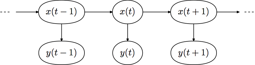
The Kalman filter is a state-space model with hidden states and observation data generated from them, similar to the hidden Markov model described previously, in which the states are continuous and changes in the state variables are statistically described using noise following a Gaussian distribution.
The Linear Dynamic System (LDS) model used in the Kalman filter is expressed by the following equation
\[p(y,x)=p(y_1|x_1)p(x_1)\displaystyle\prod_{t=2}^Tp(y_t|x_t)p(x_t|x_{t-1})\quad(1)\]
In LDS, the likelihood p(yt|xt), conditional distribution p(xt|xt-1), and prior distribution p(x1) all take the form of (multivariate) normal distributions, so the posterior distribution can be calculated analytically using forward-backward (message propagation) calculation.

We now define the stochastic generative model as follows.
\[x_0\sim Norm(\mu_0,V_0)\\x_t=A\cdot x_{t-1}+\delta_{t-1}\quad \delta_{t-1}\sim Norm(0,C)\\y_t=C\cdot x_t+\epsilon_t\quad \epsilon_t\sim Norm(0,R)\quad(2)\]
The respective varameters are as follows.
- μo: Mean value of the initial condition
- V0: Variance of the initial state
- A: Transition matrix
- Q: Transition variance matrix
- C: the observed value generator matrix
- R: the observed variance matrix
As an example, consider the task of estimating the trajectory of a noisy periodic motion in a two-dimensional latent space that gives rise to a 20-dimensional signal in the observed space. To make it periodic, we assume that the transition matrix is a simple rotation as follows and that the covariance between the transition and the observation is diagonal.
\[A=\begin{bmatrix} cos\omega&-sin\omega\\sin\omega&cos\omega\end{bmatrix}\quad Q=qI_2\quad C_{1,2}\sim Dirichlet(0.1,\dots,0.1)\quad R=rI_D\quad(3)\]
See “Getting Started with Clojure” for the Clojure environment settings and “Probabilistic Programming with Clojure” for the probabilistic programming environment settings.
First, create a project file with “lein new app gr-test (arbitrary project name)” and set the project.clj file in the project folder as follows
(defproject gr-anglican "0.1.0-SNAPSHOT"
  :description "FIXME: write description"
  :url "http://example.com/FIXME"
  :license {:name "EPL-2.0 OR GPL-2.0-or-later WITH Classpath-exception-2.0"
            :url "https://www.eclipse.org/legal/epl-2.0/"}
  :dependencies [[org.clojure/clojure "1.11.1"]
                 [anglican "1.1.0"]
                 [org.clojure/data.csv "1.0.1"]
                 [net.mikera/core.matrix "0.62.0"]
                 ;[plotly-clj "0.1.1"]
                 ;[org.nfrac/cljbox2d "0.5.0"]
                 ;[quil "3.1.0"]
                 ]
  :main ^:skip-aot gr-anglican.core
  :target-path "target/%s"
  :plugins [[org.clojars.benfb/lein-gorilla "0.6.0"]]
  :profiles {:uberjar {:aot :all
                       :jvm-opts ["-Dclojure.compiler.direct-linking=true"]}})
At the top of the directory you created, type “lein gorilla” in the terminal to run the gorilla repl server, and enter the URL displayed (http://127.0.0.1:49259(automatically generated address)/worksheet.html) in your browser to run Enter the URL ((auto-generated address)/worksheet.html) in your browser to run Gorilla Repl.
First, set up the main namespace and install the library.
(ns kalman-test
  (:require [gorilla-plot.core :as plot]
            [gorilla-repl.image :as image]
            [clojure.java.io :as io]
            [clojure.core.matrix :as mat
             :refer [matrix identity-matrix zero-vector
                     shape inverse transpose
                     mul mmul add sub div]]
            :reload)
  (:import [javax.imageio ImageIO])
  (:use [anglican core emit runtime stat]))
Next, the input data and model are set up. Set the parameters of equation (3) to ω=0.1256…, q=0.01, and r=0.01.
;; Utility

(mat/set-current-implementation :vectorz)

(def +plot-colors+ ["#05A" "#A05" "#0A5" "#50A" "#A50" "#5A0"])

;; number of time points
(def +T+ 100)
;; dimension of observation space
(def +D+ 20)
;; dimension of latent space
(def +K+ 2)

;; parameters
(def +init-state+ [0. 1.])
(def +omega+ (/ (* 4.0 Math/PI) +T+))
(def +trans-matrix+ (rotation-matrix +omega+))
(def +q+ 0.01)
(def +trans-cov+ (mul +q+ (identity-matrix +K+)))
(def +obs-matrix+
  (transpose
    (matrix
      (repeatedly 2 #(sample* (dirichlet (repeat +D+ 0.1)))))))
(def +r+ 0.01)
(def +obs-cov+ (mul +r+ (identity-matrix +D+)))
(def +init-mean+ +init-state+)
(def +init-cov+ +trans-cov+)
(def +parameters+ [+init-mean+ +init-cov+
                   +obs-matrix+ +obs-cov+
                   +trans-matrix+ +trans-cov+])

 ;; sample state sequence and observations
(def +states+
  (let [trans-dist (mvn (zero-vector +K+) +trans-cov+)]
    (reduce (fn [states _]
              (conj states
                    (add (mmul +trans-matrix+ (peek states))
                         (sample* trans-dist))))
            [+init-state+]
            (range 1 +T+))))

(def +observations+
   (let [obs-dist (mvn (zero-vector +D+) +obs-cov+)]
     (map (fn [state]
            (add (mmul +obs-matrix+ state)
                       (sample* obs-dist)))
          +states+)))
Plot the state of the latent space.
(defn get-limits
  ([points pad]
  (let [xs (mat/reshape points [(mat/ecount points)])
        x-min (reduce min xs)
        x-max (reduce max xs)
        x-pad (* pad (- x-max x-min))]
    [(- x-min x-pad) (+ x-max x-pad)]))
   ([points]
    (get-limits points 0.1)))

(def +x-limits+ (get-limits +states+))
(def +y-limits+ (get-limits +observations+))

;; plot latent states
(plot/list-plot (map #(into [] %) +states+)
                :joined true
                :color (first +plot-colors+)
                :plot-range [+x-limits+ +x-limits+])
The result plotted will be the following, noisy, circular data.

Plot the data for the first six dimensions of the observation space.
;; plot observations
(apply plot/compose
  (for [[ys color] (map vector
                        (transpose +observations+)
                        +plot-colors+)]
    (plot/list-plot ys
                    :joined true
                    :color color
                    :plot-range [:all +y-limits+])))
Based on this observed data, the parameters of the latent space are estimated. First, we set up an inference query for the Kalman filter.
(with-primitive-procedures [mmul add sub shape matrix identity-matrix zero-vector]
  (defquery kalman
    "A basic Kalman smoother. Predicts a state sequence
    from the posterior given observations"
    [observations obs-matrix obs-cov
     trans-matrix trans-cov init-mean init-cov]
    (let [;; D is dimensionality of data,
           ;; K is dimensionality of latent space
           [D K] (shape obs-matrix)
           ;; prior on observation noise
           obs-dist (mvn (zero-vector D) obs-cov)
           ;; prior on initial state
           start-dist (mvn init-mean init-cov)
           ;; prior on transition noise
           trans-dist (mvn (zero-vector K) trans-cov)]
      (matrix
        (reduce (fn [states obs]
                  (let [;; sample next state
                         prev-state (peek states)
                         state (if prev-state
                                 (add (mmul trans-matrix prev-state)
                                      (sample trans-dist))
                                 (sample start-dist))]
                    ;; observe next data point (when available)
                    (observe (count states)
                             obs-dist
                             (sub (mmul obs-matrix state) obs))
                    ;; append state to sequence and continue with next obs
                    (conj states state)))
                ;; start with empty sequence
                []
                ;; loop over data
                observations)))))
Next, we reason with them, which takes 9498.048292 msecs in a Mac M1 environment.
(def samples
  (->> (doquery :smc
             kalman
             [+observations+
              +obs-matrix+ +obs-cov+
              +trans-matrix+ +trans-cov+
              +init-mean+ +init-cov+]
             :number-of-particles 1000)
       (take 10000)
       doall
       time))
Calculate the mean and variance parameters of the posterior distribution.
(defn empirical-moments [predict-id samples]
  (let [weighted-states (collect-by predict-id samples)]
    {:mean (empirical-mean weighted-states)
     :var (empirical-variance weighted-states)}))

(def moments (empirical-moments :result samples))
Output the results.
(defn plot-moments [moments color]
  (let [mean (:mean moments)
        err (mul 2 (mat/sqrt (:var moments)))
        [T K] (shape mean)]
    (plot/compose
     (plot/list-plot (into [] (mat/slice mean 1 0))
                     :joined true
                     :plot-range [:all +x-limits+]
                     :color color)
     (plot/list-plot (into [] (mat/slice (add mean err) 1 0))
                     :plot-range [:all +x-limits+]
                     :joined true
                     :color (second +plot-colors+))
     (plot/list-plot (into [] (mat/slice (sub mean err) 1 0))
                     :plot-range [:all +x-limits+]
                     :joined true
                     :color (second +plot-colors+))
     (plot/list-plot (into [] (mat/slice mean 1 1))
                     :plot-range [:all +x-limits+]
                     :joined true
                     :color color)
     (plot/list-plot (into [] (mat/slice (add mean err) 1 1))
                     :plot-range [:all +x-limits+]
                     :joined true
                     :color (second +plot-colors+))
     (plot/list-plot (into [] (mat/slice (sub mean err) 1 1))
                     :plot-range [:all +x-limits+]
                     :joined true
                     :color (second +plot-colors+)))))
It can be confirmed that the observed data with noise is output with a certain mean and variance.
(plot-moments moments (nth +plot-colors+ 0))
For comparison, the calculation is performed with the Forward-Backward Algorithm (FBA), which is an inference algorithm for hidden Markov models.
;; Parameters (following Matlab implementation by Murphy)
;;
;; http://www.cs.ubc.ca/~murphyk/Software/Kalman/kalman.html
;;
;; m0   init-mean
;; V0   init-cov
;; C    obs-matrix
;; R    obs-cov
;; A    trans-matrix
;; Q    trans-cov

;; Filtering notation
;;
;; y    observation y(t)
;; mf   filtering expectation mf(t) = E[x(t) | y(1:t)]
;; Vf   filtering covariance Vf(t) = Cov[x(t) | y(1:t)]
;; mp   prior predictive expectation mp(t) = E[x(t) | y(1:t-1)]
;; Vp   prior predictive covariance Vp(t) = Cov[x(t) | y(1:t-1)]

(defn kalman-filter
  [observations
   obs-matrix obs-cov
   trans-matrix trans-cov
   init-mean init-cov]
  (let [;; set-up some shorthands
        C obs-matrix
        Ct (transpose C)
        R obs-cov
        A trans-matrix
        At (transpose A)
        Q trans-cov
        I (apply identity-matrix (shape init-cov))
        z (zero-vector (first (shape obs-matrix)))]
    (loop [ys observations
           mp init-mean
           Vp init-cov
           mfs []
           Vfs []
           cs []]
      (if-let [y (first ys)]
        (let [S (add (mmul C (mmul Vp Ct)) R)
              Sinv (inverse S)
              ;; K(t) = Vp(t) Ct (C Cp Ct + R)^-1
              K (mmul Vp (mmul Ct Sinv))
              ;; mf(t) = mp(t) + K(t) (y(t) - C mp(t))
              e (sub y (mmul C mp))
              mf (add mp (mmul K e))
              ;; Vf(t) = (I - K(t) C) Vp(t)
              Vf (mmul (sub I (mmul K C)) Vp)
              ;; c(t) = N(y(t) | C mp(t), C Vp Ct + R)
              c (observe* (mvn z S) e)]

          (recur (rest ys)
                 ;; mp(t+1) = A mf(t)
                 (mmul A mf)
                 ;; Vp(t+1) = A Vf At + Q
                 (add (mmul A (mmul Vf At)) Q)
                 (conj mfs mf)
                 (conj Vfs Vf)
                 (conj cs c)))
        [mfs Vfs cs]))))

;; Backward pass notation
;;
;; ms   smoothing expectation ms(t) = E[x(t) | y(1:T)]
;; Vs   smoothing covariance Vs(t) = Cov[x(t) | y(1:T)]
;; mpp  predictive expectation mpp(t) = mp(t+1) = E[x(t+1) | y(1:t)]
;;      (shifted by one relative to mp in filtering pass)
;; Vpp  predictive covariance Vpp(t) = Vp(t+1) = Cov[x(t+1) | y(1:t)]
;;      (shifted by one relative to Vp in filtering pass)

(defn kalman-backward
  [trans-matrix trans-cov mfs Vfs]
  (let [;; set-up shorthands
        A trans-matrix
        At (transpose A)
        Q trans-cov]
    (loop [mfs (pop mfs)
           Vfs (pop Vfs)
           mss (list (peek mfs))
           Vss (list (peek Vfs))]
      (if (empty? mfs)
          [mss Vss]
          (let [;; mpp(t) = mp(t+1) = A mf(t)
                mpp (mmul A (peek mfs))
                ;; Vpp(t) = Vp(t+1) = A Vf(t) At + Q
                Vpp (add (mmul A (mmul (peek Vfs) At)) Q)
                ;; J(t) = Vf(t) At Vp(t+1)^-1
                J (mmul (peek Vfs) (mmul At (inverse Vpp)))
                Jt (transpose J)
                ;; ms(t) = mf(t) + J (ms(t+1) - mp(t+1))
                ms (add (peek mfs) (mmul J (sub (peek mss) mpp)))
                ;; Vs(t) = Vf(t) + J (Vs(t+1) - Vp(t+1)) Jt
                Vs (add (peek Vfs) (mmul J (mmul (sub (peek Vfs) Vpp) Jt)))]
            (recur (pop mfs)
                   (pop Vfs)
                   (conj mss ms)
                   (conj Vss Vs)))))))

(defn kalman-smoother
  [observations
   obs-matrix obs-cov
   trans-matrix trans-cov
   init-mean init-cov]
  (let [[mfs Vfs cs] (kalman-filter observations
                       obs-matrix obs-cov
                       trans-matrix trans-cov
                       init-mean init-cov)
        [mss Vss] (kalman-backward trans-matrix trans-cov mfs Vfs)]
       [mss Vss cs]))
Calculate the mean and variance parameters of the posterior distribution using them.
(def true-moments
  (time
    (let [[mean covar _]
            (kalman-smoother +observations+
                             +obs-matrix+ +obs-cov+
                             +trans-matrix+ +trans-cov+
                             +init-mean+ +init-cov+)]
    {:mean (matrix mean)
     :var (matrix (map mat/diagonal covar))})))
Comparison of stochastic generative model and FBA. Blue is the result with the stochastic model and green is the result with FBA.
(plot/compose
  (plot/list-plot (map #(into [] %) (:mean true-moments))
                  :joined true
                  :plot-range [+x-limits+ +x-limits+]
                  :color (nth +plot-colors+ 2))
  (plot/list-plot (map #(into [] %) (:mean moments))
                  :joined true
                  :plot-range [+x-limits+ +x-limits+]
                  :color (nth +plot-colors+ 0)))
We can confirm that the trajectory of the original data is reproduced and that the results of the stochastic model and FBA are consistent.

Observational data shows similar results.
(plot-moments true-moments (nth +plot-colors+ 2))
We will now modify the original model to perform parameter estimation. One of the advantages of stochastic programming systems is that it is almost trivial to encode assumptions about the data. In this case, we can reduce the complexity of the problem by using the diagonal matrix form of A instead of estimating the full matrix, and by substituting directly into the program code using the rotated and diagonal matrix forms of Q.
(with-primitive-procedures [mmul mul add sub shape matrix identity-matrix zero-vector rotation-matrix]
  (defquery kalman-params
    "A basic Kalman smoother. Predicts a state sequence from the posterior
    given observations"
    [observations obs-matrix obs-cov init-mean init-cov]
    (let [;; D is dimensionality of data,
          ;; K is dimensionality of latent space
          [D K] (shape obs-matrix)
          ;; prior on observation noise
          obs-dist (mvn (zero-vector D) obs-cov)
          ;; prior on initial state
          start-dist (mvn init-mean init-cov)
          ;; sample transition matrix
          omega (sample (gamma 1.0 10.0))
          trans-matrix (rotation-matrix omega)
          ;; sample transition covariance
          q (sample (gamma 1.0 100.0))
          trans-cov (mul (identity-matrix K K) q)
          ;; prior on transition noise
          trans-dist (mvn (zero-vector K) trans-cov)]
      ;; loop over observations
      (reduce (fn [states obs]
                  (let [;; sample next state
                        prev-state (peek states)
                        state (if prev-state
                                  (add (mmul trans-matrix prev-state)
                                       (sample trans-dist))
                                  (sample start-dist))]
                    ;; observe next data point (when available)
                    (observe (count states)
                             obs-dist
                             (sub (mmul obs-matrix state) obs))
                    ;; append state to sequence and continue with next obs
                    (conj states state)))
                ;; start with empty sequence
                []
                ;; loop over data
                observations)
      ;; output parameters
      {:omega omega
      :q q})))
サンプル推定を行う。所要時間は9909.22075 msecsとなる。
(def param-samples
  (->> (doquery :smc
             kalman-params
             [+observations+
              +obs-matrix+ +obs-cov+
              +init-mean+ +init-cov+]
             :number-of-particles 10000)
       (take 10000)
       doall
       time))
Output an estimate of ω.” [0.12566370614359174 {:mean 0.12840811816524908, :var 8.02931252691968E-5}]” is obtained and we can deduce that the default value of 0.1256… is given with variance.
[+omega+ (empirical-moments (comp :omega :result) param-samples)]Then output an estimate of q.” [0.01 {:mean 0.013420267138197581, :var 1.564053612139262E-5}]”We can see that the default value of 0.01 is given with variance.
[+q+ (empirical-moments (comp :q :result) param-samples)]
コメント