Clojureを用いた状態空間モデル:カルマンフィルターの実装
以前”時系列データ解析(1)状態空間モデル“で述べた状態空間モデルは、主に時間軸上での変化を解析するためのツールとして用いたが、実は”隠れマルコフモデルと状態空間モデルの違いと状態空間モデルのパラメータ推定“で述べたように時間軸に特定しない状態変化の連続モデルとしても適用が可能となる。今回は状態空間モデルの応用の一つであるカルマンフィルターのClojureでの実装について述べる。
カルマンフィルターは離散的な誤差のある観測から、時々刻々と時間変化する量(例えばある物体の位置と速度)を推定するために用いられる無限インパルス応答フィルターであり、その使いやすさからレーダーやコンピュータービジョンなど幅広い工学分野で利用されている技術となる。具体的な利用例としては、機器内蔵の加速度計やGPSからの誤差のある情報を統合して、時々刻々変化する自動車の位置を推定したり、人工衛星やロケットの制御などにも用いられている。
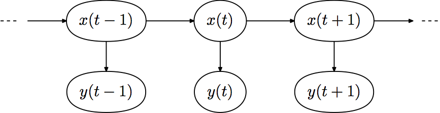
カルマンフィルターは以前述べた隠れマルコフモデル(hidden markov model)と類似した隠れ状態とそれらから生成される観測データを持つ状態空間モデルで、状態は連続であり、状態変数の変化はガウス分布に従う雑音を用いて統計的に記述されるものとなる。
カルマンフィルターに用いられるLinear Dynamic System(LDS)モデルは以下の式で表される。
\[p(y,x)=p(y_1|x_1)p(x_1)\displaystyle\prod_{t=2}^Tp(y_t|x_t)p(x_t|x_{t-1})\quad(1)\]
LDSでは尤度p(yt|xt)、条件付き分布p(xt|xt-1)、事前分布p(x1)はすべて(多変量)正規分布の形をとる為、事後分布の計算は forward-backward(メッセージ伝搬)計算により解析的に行うことができる。

ここで確率的生成モデルを以下のように定義する。
\[x_0\sim Norm(\mu_0,V_0)\\x_t=A\cdot x_{t-1}+\delta_{t-1}\quad \delta_{t-1}\sim Norm(0,C)\\y_t=C\cdot x_t+\epsilon_t\quad \epsilon_t\sim Norm(0,R)\quad(2)\]
それぞれのバラメータは以下のようになる。
- μo: 初期状態の平均値
- V0: 初期状態の分散値
- A: 遷移行列
- Q: 遷移分散行列
- C: 観測値生成行列
- R: 観測値分散行列
ここで例として、2次元の潜在空間におけるノイズ付きの周期的な運動が観測空間において20次元の信号を生じさせている場合の、2次元の潜在的空間の軌跡を推測するタスクを考える。周期性を持たせるために、遷移行列は以下のように単純な回転であり、遷移と観測の共分散は対角であると仮定する。
\[A=\begin{bmatrix} cos\omega&-sin\omega\\sin\omega&cos\omega\end{bmatrix}\quad Q=qI_2\quad C_{1,2}\sim Dirichlet(0.1,\dots,0.1)\quad R=rI_D\quad(3)\]
Clojureの環境設定は”Clojureを始めよう“を参照、確率的プログラミングの環境設定は”Clojureを用いた確率的プログラミング“を参照のこと。
まず”lein new app gr-test(任意のプロジェクト名)”でプロジェクトファイルを作成し、プロジェクトフォルダー内のproject.cljファイルを以下のように設定する。
(defproject gr-anglican "0.1.0-SNAPSHOT"
  :description "FIXME: write description"
  :url "http://example.com/FIXME"
  :license {:name "EPL-2.0 OR GPL-2.0-or-later WITH Classpath-exception-2.0"
            :url "https://www.eclipse.org/legal/epl-2.0/"}
  :dependencies [[org.clojure/clojure "1.11.1"]
                 [anglican "1.1.0"]
                 [org.clojure/data.csv "1.0.1"]
                 [net.mikera/core.matrix "0.62.0"]
                 ;[plotly-clj "0.1.1"]
                 ;[org.nfrac/cljbox2d "0.5.0"]
                 ;[quil "3.1.0"]
                 ]
  :main ^:skip-aot gr-anglican.core
  :target-path "target/%s"
  :plugins [[org.clojars.benfb/lein-gorilla "0.6.0"]]
  :profiles {:uberjar {:aot :all
                       :jvm-opts ["-Dclojure.compiler.direct-linking=true"]}})
作成したディレクトリのトップでターミナルを使って”lein gorilla”と入力し、gorilla replサーバーを動作させ、表示されたURL(http://127.0.0.1:49259(自動生成されたアドレス)/worksheet.html)をブラウザに入力してGorilla Replを動作させる。
まずメインの名前空間の設定と、ライブラリの導入を行う。
(ns kalman-test
  (:require [gorilla-plot.core :as plot]
            [gorilla-repl.image :as image]
            [clojure.java.io :as io]
            [clojure.core.matrix :as mat
             :refer [matrix identity-matrix zero-vector
                     shape inverse transpose
                     mul mmul add sub div]]
            :reload)
  (:import [javax.imageio ImageIO])
  (:use [anglican core emit runtime stat]))
次に入力データとモデルの設定を行う。(3)式のパラメータをω=0.1256…、q=0.01、r=0.01と設定する。
;; Utility

(mat/set-current-implementation :vectorz)

(def +plot-colors+ ["#05A" "#A05" "#0A5" "#50A" "#A50" "#5A0"])

;; number of time points
(def +T+ 100)
;; dimension of observation space
(def +D+ 20)
;; dimension of latent space
(def +K+ 2)

;; parameters
(def +init-state+ [0. 1.])
(def +omega+ (/ (* 4.0 Math/PI) +T+))
(def +trans-matrix+ (rotation-matrix +omega+))
(def +q+ 0.01)
(def +trans-cov+ (mul +q+ (identity-matrix +K+)))
(def +obs-matrix+
  (transpose
    (matrix
      (repeatedly 2 #(sample* (dirichlet (repeat +D+ 0.1)))))))
(def +r+ 0.01)
(def +obs-cov+ (mul +r+ (identity-matrix +D+)))
(def +init-mean+ +init-state+)
(def +init-cov+ +trans-cov+)
(def +parameters+ [+init-mean+ +init-cov+
                   +obs-matrix+ +obs-cov+
                   +trans-matrix+ +trans-cov+])

 ;; sample state sequence and observations
(def +states+
  (let [trans-dist (mvn (zero-vector +K+) +trans-cov+)]
    (reduce (fn [states _]
              (conj states
                    (add (mmul +trans-matrix+ (peek states))
                         (sample* trans-dist))))
            [+init-state+]
            (range 1 +T+))))

(def +observations+
   (let [obs-dist (mvn (zero-vector +D+) +obs-cov+)]
     (map (fn [state]
            (add (mmul +obs-matrix+ state)
                       (sample* obs-dist)))
          +states+)))
潜在空間の状態をプロットする。
(defn get-limits
  ([points pad]
  (let [xs (mat/reshape points [(mat/ecount points)])
        x-min (reduce min xs)
        x-max (reduce max xs)
        x-pad (* pad (- x-max x-min))]
    [(- x-min x-pad) (+ x-max x-pad)]))
   ([points]
    (get-limits points 0.1)))

(def +x-limits+ (get-limits +states+))
(def +y-limits+ (get-limits +observations+))

;; plot latent states
(plot/list-plot (map #(into [] %) +states+)
                :joined true
                :color (first +plot-colors+)
                :plot-range [+x-limits+ +x-limits+])
プロットされる結果は以下のような、ノイズのある円周期のデータとなる。

観察空間の最初の6次元のデータをプロットする。
;; plot observations
(apply plot/compose
  (for [[ys color] (map vector
                        (transpose +observations+)
                        +plot-colors+)]
    (plot/list-plot ys
                    :joined true
                    :color color
                    :plot-range [:all +y-limits+])))
この観測データを元に、潜在空間のパラメータを推定する。まずカルマンフィルターの推論クエリーを設定する。
(with-primitive-procedures [mmul add sub shape matrix identity-matrix zero-vector]
  (defquery kalman
    "A basic Kalman smoother. Predicts a state sequence
    from the posterior given observations"
    [observations obs-matrix obs-cov
     trans-matrix trans-cov init-mean init-cov]
    (let [;; D is dimensionality of data,
           ;; K is dimensionality of latent space
           [D K] (shape obs-matrix)
           ;; prior on observation noise
           obs-dist (mvn (zero-vector D) obs-cov)
           ;; prior on initial state
           start-dist (mvn init-mean init-cov)
           ;; prior on transition noise
           trans-dist (mvn (zero-vector K) trans-cov)]
      (matrix
        (reduce (fn [states obs]
                  (let [;; sample next state
                         prev-state (peek states)
                         state (if prev-state
                                 (add (mmul trans-matrix prev-state)
                                      (sample trans-dist))
                                 (sample start-dist))]
                    ;; observe next data point (when available)
                    (observe (count states)
                             obs-dist
                             (sub (mmul obs-matrix state) obs))
                    ;; append state to sequence and continue with next obs
                    (conj states state)))
                ;; start with empty sequence
                []
                ;; loop over data
                observations)))))
次にそれらを用いて推論する。Mac M1環境で9498.048292 msecsかかる。
(def samples
  (->> (doquery :smc
             kalman
             [+observations+
              +obs-matrix+ +obs-cov+
              +trans-matrix+ +trans-cov+
              +init-mean+ +init-cov+]
             :number-of-particles 1000)
       (take 10000)
       doall
       time))
事後分布の平均と分散パラメータを計算する。
(defn empirical-moments [predict-id samples]
  (let [weighted-states (collect-by predict-id samples)]
    {:mean (empirical-mean weighted-states)
     :var (empirical-variance weighted-states)}))

(def moments (empirical-moments :result samples))
結果を出力する。
(defn plot-moments [moments color]
  (let [mean (:mean moments)
        err (mul 2 (mat/sqrt (:var moments)))
        [T K] (shape mean)]
    (plot/compose
     (plot/list-plot (into [] (mat/slice mean 1 0))
                     :joined true
                     :plot-range [:all +x-limits+]
                     :color color)
     (plot/list-plot (into [] (mat/slice (add mean err) 1 0))
                     :plot-range [:all +x-limits+]
                     :joined true
                     :color (second +plot-colors+))
     (plot/list-plot (into [] (mat/slice (sub mean err) 1 0))
                     :plot-range [:all +x-limits+]
                     :joined true
                     :color (second +plot-colors+))
     (plot/list-plot (into [] (mat/slice mean 1 1))
                     :plot-range [:all +x-limits+]
                     :joined true
                     :color color)
     (plot/list-plot (into [] (mat/slice (add mean err) 1 1))
                     :plot-range [:all +x-limits+]
                     :joined true
                     :color (second +plot-colors+))
     (plot/list-plot (into [] (mat/slice (sub mean err) 1 1))
                     :plot-range [:all +x-limits+]
                     :joined true
                     :color (second +plot-colors+)))))
ノイズを含んだ観察データがある平均値と分散を持った出力になっていることが確認できる。
(plot-moments moments (nth +plot-colors+ 0))
比較の為に隠れマルコフモデルの推論アルゴリズムであるForward-Backward Algorithm(FBA)での計算を行う。
;; Parameters (following Matlab implementation by Murphy)
;;
;; http://www.cs.ubc.ca/~murphyk/Software/Kalman/kalman.html
;;
;; m0   init-mean
;; V0   init-cov
;; C    obs-matrix
;; R    obs-cov
;; A    trans-matrix
;; Q    trans-cov

;; Filtering notation
;;
;; y    observation y(t)
;; mf   filtering expectation mf(t) = E[x(t) | y(1:t)]
;; Vf   filtering covariance Vf(t) = Cov[x(t) | y(1:t)]
;; mp   prior predictive expectation mp(t) = E[x(t) | y(1:t-1)]
;; Vp   prior predictive covariance Vp(t) = Cov[x(t) | y(1:t-1)]

(defn kalman-filter
  [observations
   obs-matrix obs-cov
   trans-matrix trans-cov
   init-mean init-cov]
  (let [;; set-up some shorthands
        C obs-matrix
        Ct (transpose C)
        R obs-cov
        A trans-matrix
        At (transpose A)
        Q trans-cov
        I (apply identity-matrix (shape init-cov))
        z (zero-vector (first (shape obs-matrix)))]
    (loop [ys observations
           mp init-mean
           Vp init-cov
           mfs []
           Vfs []
           cs []]
      (if-let [y (first ys)]
        (let [S (add (mmul C (mmul Vp Ct)) R)
              Sinv (inverse S)
              ;; K(t) = Vp(t) Ct (C Cp Ct + R)^-1
              K (mmul Vp (mmul Ct Sinv))
              ;; mf(t) = mp(t) + K(t) (y(t) - C mp(t))
              e (sub y (mmul C mp))
              mf (add mp (mmul K e))
              ;; Vf(t) = (I - K(t) C) Vp(t)
              Vf (mmul (sub I (mmul K C)) Vp)
              ;; c(t) = N(y(t) | C mp(t), C Vp Ct + R)
              c (observe* (mvn z S) e)]

          (recur (rest ys)
                 ;; mp(t+1) = A mf(t)
                 (mmul A mf)
                 ;; Vp(t+1) = A Vf At + Q
                 (add (mmul A (mmul Vf At)) Q)
                 (conj mfs mf)
                 (conj Vfs Vf)
                 (conj cs c)))
        [mfs Vfs cs]))))

;; Backward pass notation
;;
;; ms   smoothing expectation ms(t) = E[x(t) | y(1:T)]
;; Vs   smoothing covariance Vs(t) = Cov[x(t) | y(1:T)]
;; mpp  predictive expectation mpp(t) = mp(t+1) = E[x(t+1) | y(1:t)]
;;      (shifted by one relative to mp in filtering pass)
;; Vpp  predictive covariance Vpp(t) = Vp(t+1) = Cov[x(t+1) | y(1:t)]
;;      (shifted by one relative to Vp in filtering pass)

(defn kalman-backward
  [trans-matrix trans-cov mfs Vfs]
  (let [;; set-up shorthands
        A trans-matrix
        At (transpose A)
        Q trans-cov]
    (loop [mfs (pop mfs)
           Vfs (pop Vfs)
           mss (list (peek mfs))
           Vss (list (peek Vfs))]
      (if (empty? mfs)
          [mss Vss]
          (let [;; mpp(t) = mp(t+1) = A mf(t)
                mpp (mmul A (peek mfs))
                ;; Vpp(t) = Vp(t+1) = A Vf(t) At + Q
                Vpp (add (mmul A (mmul (peek Vfs) At)) Q)
                ;; J(t) = Vf(t) At Vp(t+1)^-1
                J (mmul (peek Vfs) (mmul At (inverse Vpp)))
                Jt (transpose J)
                ;; ms(t) = mf(t) + J (ms(t+1) - mp(t+1))
                ms (add (peek mfs) (mmul J (sub (peek mss) mpp)))
                ;; Vs(t) = Vf(t) + J (Vs(t+1) - Vp(t+1)) Jt
                Vs (add (peek Vfs) (mmul J (mmul (sub (peek Vfs) Vpp) Jt)))]
            (recur (pop mfs)
                   (pop Vfs)
                   (conj mss ms)
                   (conj Vss Vs)))))))

(defn kalman-smoother
  [observations
   obs-matrix obs-cov
   trans-matrix trans-cov
   init-mean init-cov]
  (let [[mfs Vfs cs] (kalman-filter observations
                       obs-matrix obs-cov
                       trans-matrix trans-cov
                       init-mean init-cov)
        [mss Vss] (kalman-backward trans-matrix trans-cov mfs Vfs)]
       [mss Vss cs]))
それらを用いた事後分布の平均と分散パラメータを計算する。
(def true-moments
  (time
    (let [[mean covar _]
            (kalman-smoother +observations+
                             +obs-matrix+ +obs-cov+
                             +trans-matrix+ +trans-cov+
                             +init-mean+ +init-cov+)]
    {:mean (matrix mean)
     :var (matrix (map mat/diagonal covar))})))
確率的生成モデルとFBAの比較を行う。青が確率モデルを用いたもの、緑がFBAでの結果となる。
(plot/compose
  (plot/list-plot (map #(into [] %) (:mean true-moments))
                  :joined true
                  :plot-range [+x-limits+ +x-limits+]
                  :color (nth +plot-colors+ 2))
  (plot/list-plot (map #(into [] %) (:mean moments))
                  :joined true
                  :plot-range [+x-limits+ +x-limits+]
                  :color (nth +plot-colors+ 0)))
元のデータの軌跡を再現し、かつ確率モデルとFBAの結果は一致することが確認できる。

観測データを見ても同様な結果となっている。
(plot-moments true-moments (nth +plot-colors+ 2))
ここで、パラメータ推定を行うために、元のモデルを修正することにする。確率的プログラミングシステムの利点の一つは、データに関する仮定を符号化するのがほとんど些細なことであることです。この場合、我々は完全な行列を推定する代わりに、Aの対角行列形式を使い、Qの回転行列形式と対角行列形式を使ってプログラムコードに直接代入することにより、問題の複雑さを軽減することができる。
(with-primitive-procedures [mmul mul add sub shape matrix identity-matrix zero-vector rotation-matrix]
  (defquery kalman-params
    "A basic Kalman smoother. Predicts a state sequence from the posterior
    given observations"
    [observations obs-matrix obs-cov init-mean init-cov]
    (let [;; D is dimensionality of data,
          ;; K is dimensionality of latent space
          [D K] (shape obs-matrix)
          ;; prior on observation noise
          obs-dist (mvn (zero-vector D) obs-cov)
          ;; prior on initial state
          start-dist (mvn init-mean init-cov)
          ;; sample transition matrix
          omega (sample (gamma 1.0 10.0))
          trans-matrix (rotation-matrix omega)
          ;; sample transition covariance
          q (sample (gamma 1.0 100.0))
          trans-cov (mul (identity-matrix K K) q)
          ;; prior on transition noise
          trans-dist (mvn (zero-vector K) trans-cov)]
      ;; loop over observations
      (reduce (fn [states obs]
                  (let [;; sample next state
                        prev-state (peek states)
                        state (if prev-state
                                  (add (mmul trans-matrix prev-state)
                                       (sample trans-dist))
                                  (sample start-dist))]
                    ;; observe next data point (when available)
                    (observe (count states)
                             obs-dist
                             (sub (mmul obs-matrix state) obs))
                    ;; append state to sequence and continue with next obs
                    (conj states state)))
                ;; start with empty sequence
                []
                ;; loop over data
                observations)
      ;; output parameters
      {:omega omega
      :q q})))
サンプル推定を行う。所要時間は9909.22075 msecsとなる。
(def param-samples
  (->> (doquery :smc
             kalman-params
             [+observations+
              +obs-matrix+ +obs-cov+
              +init-mean+ +init-cov+]
             :number-of-particles 10000)
       (take 10000)
       doall
time))ωの推定値を出力する。”[0.12566370614359174 {:mean 0.12840811816524908, :var 8.02931252691968E-5}]”が得られ、初期設定値である0.1256…が分散を持って与えられていることが推論できる。
[+omega+ (empirical-moments (comp :omega :result) param-samples)]次にqの推定を出力する。”[0.01 {:mean 0.013420267138197581, :var 1.564053612139262E-5}]”初期設定値である0.01が分散を持って与えられていることが確認できる。
[+q+ (empirical-moments (comp :q :result) param-samples)]
AIシステム設計・意思決定構造の設計を専門としています。
Ontology・DSL・Behavior Treeによる判断の外部化、マルチエージェント構築に取り組んでいます。
Specialized in AI system design and decision-making architecture.
Focused on externalizing decision logic using Ontology, DSL, and Behavior Trees, and building multi-agent systems.
