LINE(Large-scale Information Network Embedding)
LINE (Large-scale Information Network Embedding) is a type of graph data algorithm that can be used to efficiently embed a large-scale information network (graph) of about 1 million nodes at high speed (in a few hours on a regular PC). The method optimizes an objective function that preserves the local and global graph structure, and also targets directed and undirected graphs and weighted graphs.
LINE, reported in “LINE: Large-scale Information Network Embedding” by members from Microsoft, Peking University, and the University of Michigan, aims to learn feature vectors (embeddings) of nodes (nodes represent individual elements or entities in a graph). These feature vectors can be used to capture relationships and similarities between nodes and can be applied to a variety of tasks.
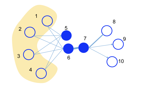
We will now discuss the primary and secondary proximity, which is a feature of LINE.

In the above figure, node 5 and node 6 are not connected by an edge, but they are indirectly connected via node 1 to node 4, so the relationship between the two nodes is considered strong.
Conventional graph embedding methods such as multidimensional scaling (MDS), Isomap, Laplacian, and Eigenmap (LE, Laplacian eigenmap) require the computation of the principal eigenvectors of the adjacency matrix, which generally requires more than \(O(N^3)\)} when the number of nodes is N. or more when the number of nodes is N, which makes the computation difficult for large graphs.
In contrast, the above paper lists the following characteristics of LINe.
- LINEe is a new graph embedding that can be extended to millions of nodes, even for directed and weighted graphs.
- An objective function that preserves both first-order and second-order proximity is designed, and an edge sampling algorithm is developed for optimization. The limitations of conventional stochastic gradient descent methods are overcome, and the effectiveness and efficiency of inference are improved.
- Experiments were conducted on real-world information networks to demonstrate its usefulness.
The main features of LINE are as follows.
1. edge type learning: LINE can learn different embeddings between different types of edges (links). This is useful when different types of links have different meanings in a graph.
2. high-dimensional embedding: LINE typically represents nodes in a high-dimensional embedding space. While high-dimensional embeddings facilitate the capture of fine-grained similarities between nodes, they are also computationally expensive.
3. relevance to neighboring nodes: LINE is designed to optimize the degree to which each node is related to its immediate neighbors. This information helps determine the position of a node in the graph.
4. improved computational efficiency: LINE is designed to be computationally efficient for large graphs. For example, it uses Negative Sampling to reduce computational cost.
LINE can be used in a variety of tasks related to graph data, such as computing node similarity, node classification, link prediction, and recommendation systems. graph embedding algorithms such as LINE can be used in social network analysis, bioinformatics, information retrieval, online advertising, reputation analysis, fraud detection, and many other applications.
Algorithms used in LINE (Large-scale Information Network Embedding)
The problem definition in LINE is as follows. The edges\(e\in \mathbf{G}=(\mathbf{V},\mathbf{E})\) in the graph\(\mathbf{G}=(\mathbf{V},\mathbf{E})\) are ordered pairs of nodes e=(u,v), each with a non-negative weight\(\omega_{u,v}\gt 0\). First-order proximity is the local proximity between two nodes, and the first-order proximity of nodes u and v connected by edge (u,v) is weighted\(\omega_{uv}\). First-order proximity represents the similarity of nodes, but in real-world graphs, some observed edges are missing and many are not. Therefore, first-order proximity alone is not sufficient, and it is necessary to consider proximity through common friends, as in the case of friendship.
Second-order proximity is the similarity between nodes u and v and their neighbors connected by edges. If the first-order proximity between node u and all other nodes is \(p_u=(\omega_{u,1},\omega_{u,2},\dots,\omega_{u,|V|})\), the second-order proximity between node u and node v is the similarity between \(p_u\) and \(p_v\). If no node is connected by an edge to both u and v, then the second-order proximity of node u and node v is zero.
As a model for first-order proximity, for each undirected edge (i,j), the join probability is defined as follows.
\[p_1(v_i,v_j)=\frac{1}{1+e^{-\vec{u}_i^T\cdot\vec{u}_j}}\]
where \(\vec{U}_i\in\mathbb{R}^d\) is the low-dimensional vector representation of node\(v_i\).
The above equation defines the distribution of \(\mathbf{V}\times\mathbf{V}\) space, whose empirical probability is \(\hat{p}_1(i,j)=\frac{\omega_{ij}}{\mathbf{W}} \left(but\mathbf{W}=\sum_{(i, A straightforward way to maintain first-order proximity is to minimize the following objective function
\[O_1=d(\hat{p}_1(\cdot , \cdot),\ p_1(\cdot , \cdot))\]
where d(⋅, ・) is the distance between the two distributions. Replacing this d by KL-divergence and removing the constant yields the following equation.
\[O_1=-\displaystyle\sum_{(i,j)\in E}\omega_{ij}log p_1(v_i,v_j)\]
By finding the \(\{\vec{u}_i\}_{i=1\dots |V|}\) that minimizes this expression, we can represent each node in d dimensions.
Second-order proximity is defined under the assumption that nodes that share a bond with many other nodes are similar to each other. Each node has two roles: as a node itself and as a context for other nodes. For node\(v_i\), we introduce two vectors\(\vec{u}_i\) and\(\vec{u}_i’\). The former is a representation of the node \(v_i\) itself, while the latter is a representation as a context. For each directed edge (i, j), we define the probability of the context of \(v_j\) created by node\(v_i\) as follows.
\[p_2(v_j|v_i)=\frac{e^{\vec{u’}^T\cdot\vec{u}_i}}{\sum_{k=1}^{|V|}e^{\vec{u’}_k^T\cdot \vec{u}_i}}\]
where is the number of nodes|V|(context).
For each node, the above formula defines a conditional probability distribution \(p_2(\cdot |v_i)\) for the context (the set of all nodes in the network). In order to maintain second-order proximity, the conditional probability distribution\(p_2(\cdot |v_i)\) of the context, which is a low-dimensional representation, must be close to the empirical probability\(\hat{p}_2(\cdot |v_i)\). Therefore, the following objective function is minimized.
\[O_2=\displaystyle\sum_{i\in V}\lambda_i d(\hat{p}_2(\cdot |v_i),\ p_2(\cdot |v_i))\]
Here it is the distance between the two distributions. Since the importance of nodes in a graph generally differs, we can express the importance of node i in the graph by introducing \(\lambda_i\) in the objective function. Specifically, it is expressed in terms of degree and page rank (PageRank). The empirical probability \(\hat{p}_2(\cdot | v_i)\) is defined by \(\hat{p}_2(v_j | v_i)=\frac{\omega_{ij}}{d_i}\). where is the weight of edge (i, j), \(d_i\) is the outgoing order of node i (\(d_i=\sum_{k\in N(i)}\omega_{ik}\) and N(i) is the set of neighborhoods by edges from node i to other nodes). In LINE, for simplicity, we assume that \(\lambda_i=d_i\). KL-divergence is used as the distance function between the distributions. Replacing d(||.) with KL-divergence in the above equation and eliminating the constant as \(\lambda_i=d_i\), we obtain the following equation.
\[O_2=-\displaystyle\sum_{(i,j)\in E}\omega_{ij}log p_2(v_j|v_i)\]
By learning the \(\{\vec{u}_i\}_{i=1,\dots,|V|}\) and \(\{\vec{u}_i’\}_{i=1,\dots,|V|}\) that minimize this objective function, we can represent each node\(v_i\) by a d-dimensional vector\(\vec{u}_i\) . A simple and effective way to achieve embeddings that preserve first-order and second-order proximity is to train those that preserve first-order proximity and those that preserve second-order proximity separately and combine the embeddings for each vertex obtained with each. The method of optimizing both objective functions at the same time is a subject for future work. The optimization of the above equation is computationally expensive because it is necessary to calculate the sum over all node sets when calculating the conditional probability \(p_2(\cdot |v_i)\). To solve this problem, NEGATIVE SAMPLING is performed according to the noise distribution of each edge (i, j). Since the computational complexity of LINE is proportional to the number of edges (|E|) and independent of the number of nodes (|V|), LINE is faster than other methods in large networks.
LINE is able to comprehensively capture node similarity and relatedness, making it an effective algorithm for generating effective embeddings for large-scale information networks, and this embedding can be applied to a variety of graph data-related tasks.
“LINE: Large-scale Information Network Embedding” uses linguistic networks (Wikipedia), social networks (Flicker and YouTube), and citation networks (BDLP) as experiments to generate effective embeddings for Graph Fractorization, DeepWalk described in “DeepWalk Overview, Algorithms, and Example Implementations,”, and SkipGram on linguistic analogy and document classification tasks.
The code is available on a git page by the author.
Example implementation of LINE (Large-scale Information Network Embedding)
LINE (Large-scale Information Network Embedding) is an algorithm for embedding graph data, but its implementation depends on programming languages and libraries. The following is an example of LINE implementation using Python and a general machine learning library.
import numpy as np
import networkx as nx
from gensim.models import Word2Vec

# Loading Graphs
G = nx.read_edgelist("graph.txt", create_using=nx.Graph())

# Line implementation
def LINE(graph, dimensions, walk_length, num_walks):
    walks = []
    for _ in range(num_walks):
        for node in graph.nodes():
            walk = random_walk(graph, node, walk_length)
            walks.append(walk)

    model = Word2Vec(walks, vector_size=dimensions, sg=1, hs=1)

    return model

def random_walk(graph, start_node, walk_length):
    walk = [start_node]
    while len(walk) < walk_length:
        neighbors = list(graph.neighbors(walk[-1]))
        if len(neighbors) == 0:
            break
        next_node = np.random.choice(neighbors)
        walk.append(next_node)
    return [str(node) for node in walk]

# LINE CALL
dimensions = 128
walk_length = 10
num_walks = 100
line_model = LINE(G, dimensions, walk_length, num_walks)

# Get Embedded Vector
node_embeddings = {node: line_model.wv[str(node)] for node in G.nodes()}
In this example implementation, the following steps are performed
- Load graph data. Although the networkx library is used here, the graph should be read in an appropriate way depending on the format of the data.
- Implement the LINE algorithm. Perform a random walk and feed it into the Word2Vec model to learn node embeddings The LINE algorithm performs a random walk of the graph and learns it as a Word2Vec to generate embedding vectors for the nodes.
- Obtain the embedding vectors; use the LINE model to extract the embedding vectors for each node.
Challenge for LINE (Large-scale Information Network Embedding)
LINE (Large-scale Information Network Embedding) is an excellent graph embedding algorithm, but there are some challenges and limitations. These issues are described below.
1. Computational cost: LINE learns in a high-dimensional embedding space, which can be computationally expensive for large graphs. In particular, when considering 2nd-order proximity (2nd-Order Similarity), the computation explodes when the number of common neighbors is large.
2. adjustment of hyper-parameters: LINE has several hyper-parameters (embedding dimension, walk length, number of walks, etc.), and adjustment of these parameters is necessary. The choice of appropriate hyperparameters depends on the task and may need to be adjusted manually.
3. support for non-homogeneous graphs: LINE is suitable for homogeneous graphs (graphs with a single node type and a single edge type) and may be difficult to apply to non-homogeneous graphs (graphs with multiple node types and edge types). For non-homogeneous graphs, relevance to different node types and edge types should be considered.
4. Application to stream data: LINE is designed for static graphs and may be difficult to apply to dynamic stream data. If the graph changes over time, LINE embedding may not be able to keep up.
5. scalability: LINE is designed to efficiently learn embeddings for large graphs, but it may still be difficult to apply to some very large graphs. Faster and more scalable algorithms are required.
Measures to Address the Challenges of LINE (Large-scale Information Network Embedding)
Several measures can be taken to address the challenges of LINE (Large-scale Information Network Embedding). The following describes measures to address the main issues of LINE.
1. addressing the computational costs:
Mini-batch learning: When performing random walks, instead of processing all walks at once, mini-batch learning can be introduced to reduce computational cost. This method allows for efficient learning even on large graphs.
2. addressing hyper-parameter tuning:
Automatic Tuning: Hyperparameter auto-tuning tools can be used to find optimal settings for hyperparameters. For example, Bayesian optimization or grid search can be used to find the optimal parameters.
3. dealing with non-homogeneous graphs:
Model Extension: In order to deal with non-homogeneous graphs, the LINE model can be extended. This allows incorporating information about different node types and edge types, e.g., considering methods such as Metapath2Vec.
4. coping with streamed data:
Dynamic graph embedding: If graphs change over time, dynamic graph embedding algorithms can be considered. For example, algorithms such as DynamicLINE and GraphSAGE described in “Overview of GraphSAGE, Algorithms, and Examples of Implementations. Algorithms and Examples of Implementations” are suitable for stream data.
5. addressing scalability:
Distributed Processing: To deal with large graphs, distributed processing frameworks can be used. For example, Apache Spark and graph databases can be leveraged to increase processing power.
6. graph sampling:
Another way to reduce computational cost is to sample and process large graphs into subgraphs. In a random walk, a random walk of subgraphs could be performed.
7. use of state-of-the-art algorithms:
It will be important to consider improved versions of LINE and other graph embedding algorithms. New algorithms are frequently proposed in the field of graph data analysis, and it will be beneficial to select the best algorithm for the task.
Reference Information and Reference Books
For more information on graph data, see “Graph Data Processing Algorithms and Applications to Machine Learning/Artificial Intelligence Tasks. Also see “Knowledge Information Processing Techniques” for details specific to knowledge graphs. For more information on deep learning in general, see “About Deep Learning.
Reference book is

“Graph Neural Networks: Foundations, Frontiers, and Applications“等がある。

“Introduction to Graph Neural Networks“

“Graph Neural Networks in Action“


コメント