Overview of the epsilon-greedy method
The ε-greedy method (ε-greedy) is a simple and effective strategy for dealing with the trade-off between exploration and exploitation (exploitation and exploitation), such as reinforcement learning, where the algorithm adjusts the probability of selecting an optimal action and the probability of selecting a random action This will be the method to be used in the following section.

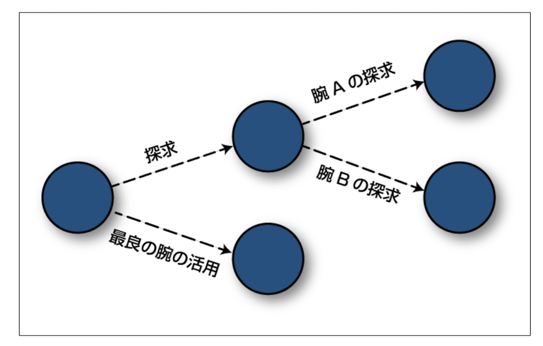
An overview of the ε-Greedy method is given below.
- The ε-Greedy method uses a parameter called ε (epsilon), where ε takes values between 0 and 1.
- The ε-Greedy method balances the probability of an agent choosing the optimal action as ε and the probability of choosing a random action (search) as 1-ε.
- The ε-Greedy method can adjust the balance between exploration and exploitation depending on the value of ε. When ε is small, the agent primarily chooses known optimal actions, and when ε is large, the agent tries random actions frequently.
- The ε-Greedy method emphasizes exploration in the initial phase, exploring the environment to gather new information. However, as time passes, ε is reduced, making it easier to use the information collected to choose the optimal action.
- The ε-Greedy method is widely used in reinforcement learning tasks to learn optimal strategies. It is employed as a search strategy in many reinforcement learning algorithms (e.g., Q-Learning described in “Overview of Q-Learning, Algorithms and Examples of Implementations” and SARSA described in “Overview of SARSA, Algorithms and Implementation Systems“).
The epsilon-Greedy method is a practical approach for many reinforcement learning tasks because it allows for an adjustable balance between exploration and exploitation.
Specific procedures for the epsilon-greedy method (epsilon-greedy)
The ε-greedy method (ε-greedy) is a general method for managing the trade-off between search and exploitation in reinforcement learning, in which the method selects a random action with ε probability and the current optimal action with 1-ε probability. The specific steps of the ε-Greedy method are described below.
First, the following can be defined as a class of objects representing epsilon-greedy.
class EpsilonGreedy ():
   def __init__(self, epsilon, counts, value):
      self.epsilon = epsilon
      self.counts = counts
      self.values = values
   return
Here, epsilon indicates how often a given arm is searched for and is defined as a floating-point number (e.g., if epsilon=0.1, 10% of the number of times an arm is searched for will be applied to the arm search), counts indicates how many times each of the N arms given as a vector of length N is searched for in the current bandit problem (e.g., arms1 and arm2, each run twice, counts=[2,2]), and values is a floating-point vector that is the average of the rewards for each of the given N arms (e.g., arm1 is run once for 1 unit, another run for 0 units, and arm2 is run once for 1 unit, and arm2 is run once for 0 units). 0 units rewarded, and arm2, 0 units rewarded for 2 plays, values=[0.5, 0.0])
1. Initialization:
- Initialize value and reward estimates for each action in the reinforcement learning problem. These estimates provide an indication of how good each behavior is.
def initialize(self, n-arms):
  self.counts = [0 for col in range(n_srms)]:
  self.values = [0.0 for col in range(n-arms)]
return
2. action selection:
- Select a random action with a probability of ε. This encourages exploration by trying new behaviors.
- Select the behavior with a probability of 1-ε that has the highest current estimate of value or reward. This leverages known good behaviors.
def ind_max(x):
  m = max(x)
return x.index(m)

def select_arm(self):
  if random.random() > self.epsilon:
     return ind_max(self.values)
  else:
     return random.randrange(len(self.values))
In the above code, if the randomly generated number is greater than epsilon, the algorithm selects the arm with the largest cache value in the value field, otherwise it selects the arm at random.
3. observe rewards and update estimates:
- Observe the actual reward for the selected behavior.
- Update estimates. This is a method of bringing the estimate of the selected behavior closer to the actual reward, e.g., moving average or time series update methods may be used.
def update(self, chosen_arm, reward):
  self.counts[chosen_arm] = self.count[chosen_arm] + 1
  n = self.count[chosen_arm]

  value = self.values[chosen_arm]
  new_value = ((n-1) / float(n)) * value + (1 / float(n)) * reward
  self.values[chosen_arm] = new_value
return
In the above code, UPDATE increases COUNTS to check the current estimate of the selected arm, and if it is the first time, it updates the reward received for drawing that arm, and if it is an arm that has been drawn in the past, it updates the estimate of the selected arm as a weighted average of the previous estimate and the reward just received.
This indicates that if there is more experience with a particular choice, the value of one observation becomes less and less valuable to the algorithm. This weighting factor becomes an important parameter when the reward for pulling an arm varies over time.
4. iterative:
- Repeat the above steps iteratively. As the system learns, the ε-Greedy method is expected to find the optimal behavior, balancing exploration and exploitation.
The ε-Greedy method can explore unknown states and behaviors through exploration and at the same time use known information to learn efficiently. By adjusting the value of ε, the ratio of exploration and utilization can be changed, making it a fluid method. For example, a smaller value of ε emphasizes more utilization, while a larger value of ε results in more exploration.
Example implementation of the epsilon-greedy method (epsilon-greedy)
An example implementation of the ε-greedy method (ε-greedy) is shown. In this example, the value of ε is set to 0.1 (10% probability of selecting a random action) and is used in combination with Q-learning. The following is an example of Python code.
import random

# Initialize Q table (set number of states and actions as an example)
num_states = 10
num_actions = 4
Q = [[0 for _ in range(num_actions)] for _ in range(num_states)]

# Epsilon setting
epsilon = 0.1  # Set the value of epsilon to 0.1

# Parameters of Q study (learning rate and discount rate)
learning_rate = 0.1
discount_factor = 0.9

# Number of episodes
num_episodes = 1000

# Perform Q-learning
for episode in range(num_episodes):
    state = random.randint(0, num_states - 1)  # Random initial condition

    while True:
        # Action selection by epsilon-Greedy method
        if random.uniform(0, 1) < epsilon:
            action = random.randint(0, num_actions - 1)  # Random action selected with epsilon probability
        else:
            action = Q[state].index(max(Q[state]))  # 1 - Select the optimal action with ε probability

        # Perform actions to obtain the next state and reward
        next_state = random.randint(0, num_states - 1)  # Next state of dummy
        reward = 0  # Dummy Rewards

        # Q value update (Q learning)
        best_next_action = Q[next_state].index(max(Q[next_state]))
        Q[state][action] = Q[state][action] + learning_rate * (reward + discount_factor * Q[next_state][best_next_action] - Q[state][action])

        state = next_state

        if state == num_states - 1:
            break

# Display of study results
print("Learning results (Q table):")
for i in range(num_states):
    print("condition", i, ":", Q[i])
This code implements Q learning using the ε-Greedy method, where random search and utilization of optimal behavior is tuned based on the value of ε. The value of ε and other parameters can be tuned depending on the problem, and although this example is applied to Q learning, the ε-Greedy method can be applied to other reinforcement learning algorithms as well.
Debugging the code for the epsilon-greedy method (epsilon-greedy)
In the Bandit algorithm, the algorithm actively chooses the data it should receive and uses it to learn online. Therefore, compared to general machine learning algorithms that do not actively learn, it is necessary to debug the algorithm in a way that allows it to operate on its own to some extent, rather than simply providing it with data.
The method often used to achieve these goals is Monte Carlo simulation. For example, one might assume that every time someone sees an ad, there is a fixed probability that he or she will click on it, and use a bandit algorithm to estimate this probability and determine a strategy to maximize the click-through rate, or if a new visitor, who is not a registered user, visits the site, there is a fixed probability that he or she will click on a landing page, If a new visitor, who is not a registered user, visits the site, and is assumed to have a fixed probability of viewing the landing page and registering as a user, the problem is to estimate this probability and determine a strategy to maximize the conversion rate.
Such a problem can be created by assuming an establishment distribution (Bernoulli distribution) where the reward is 1 for a certain time and 0 for the rest of the time.
For example, when a potential user visits the site, he/she selects an arm and is presented with a particular web structure, and the visitor then chooses whether to register as a user (receiving a reward of 1) or not (receiving a reward of 0). Such a simulation is called the Bernoulli arm and is represented by the following code.
class BernouliArm():
  def __init__(self, p):
    self.p = p

  def draw(self):
    if random.random() > self.p:
       return 0.0
    else:
       return 1.0
To apply this approach to a number of arms to be processed, do the following
means = [0.1, 0.1, 0.1, 0.1, 0.9]
n_arms = len(means)
random.shuffle(means)
arms = map(lambda (mu): BernouliArm(mu), means)
This approach sets up an array with five arms, four of which produce a 10% time reward, while the best arm is the one that produces a 90% time reward. To test the Bernoulli arms, draw is called several times for several elements of the array.
The test algorithm using these is as follows.
def test_algorithm(algo, arms, num_sims, horizon):
  chosen_arms = [0.0 for i in range(num_sims * horizon)]
  rewards = [0.0 for i in range(num_sims * horizon)]
  cumulative_rewards = [0.0 for i in range(num_sims * horizon)]
  sim_nums = [0.0 for i in range(num_sims * horizon)]
  times = [0.0 for i in range(num_sims * horizon)]

  for sim in range(num_sims):
    sim = sim + 1
    algo.initialize(len(arms))

    for t in range(horizon):
      t = t + 1
      index = (sim - 1) * horizon + t - 1
      sim_nums[index] = sim
      times[index] = t

      chosen_arm = algo.select_arm()
      chosen_arms[index] = chosen_arm

      reward = arms[chosen_arms[index]].draw()
      rewards[index] = reward

      if t == 1:
        cumulative_rewards[index] = reward
      else:
        cumulative_rewards[index] = cumulative_rewards[index - 1] + reward

      algo.update(chosen_arm, reward)

  return [sim_nums, times, chosen_arms, rewards, cumulative_rewards]
The results of evaluating the epsilon-greedy method (ε-greedy) in these test cases are shown below.

Those with large epsilon (more time is allocated to search) start up faster. The smaller the value, the slower the start-up, but the higher the final performance level achieved.
However, in terms of cumulative rewards, those with smaller epsilon are not higher because they take more bad choices.

Challenges of the epsilon-greedy method (ε-greedy)
The ε-greedy method (ε-greedy) is a powerful strategy for reconciling the trade-off between search and exploitation in reinforcement learning, but several challenges exist. The following are the main challenges of the ε-greedy method.
1. fixed ε-parameters:
The ε-Greedy method usually uses fixed ε parameters. However, the optimal value of ε may vary depending on the nature of the problem, and a fixed ε parameter may not achieve the optimal balance between search and utilization.
2. rate of decrease of ε:
Choosing the rate of decrease of ε (the rate at which ε decreases over time) is a challenging task and requires trial and error to find the right speed. If the speed is too fast, utilization is prioritized early on and exploration may be lacking. If the speed is too slow, the search will continue for a long time and convergence may be slow.
3. knowledge of optimal ε is required:
The ε-Greedy method assumes a priori knowledge of the optimal ε value. However, finding the optimal ε in an unknown environment or task can be difficult.
4. wasted search when ε is high:
When ε is high, the agent frequently chooses random actions. This increases the amount of wasted search in learning and may reduce learning efficiency.
5. effect of randomness:
The ε-Greedy method has a stochastic component. Therefore, if the same ε-Greedy method is run multiple times in different environments and seeds, the results may differ.
To address these challenges, parameter tuning of the ε-Greedy method, adoption of derived algorithms, automatic hyperparameter tuning, dynamic adjustment of ε (e.g., ε diminishing), and combinations of various search strategies may be used. The optimal search strategy depends on the specific task and environment and must be found through experimentation and adjustment.
Addressing the Challenges of the ε-Greedy Method (ε-Greedy)
The following is a description of how to address the challenges of the ε-Greedy method.
1. ε adjustment:
In the ε-Greedy method, it is important to adjust the value of ε. If ε is too small, the search will be insufficient, and if ε is too large, unnecessary random actions will increase. To find the optimal value of ε, there is a way to adjust the value of ε over time, decreasing ε and emphasizing exploration in the early stages of learning and increasing utilization in later stages.
2. sequential ε adjustment:
In the ε-Greedy method, the value of ε must be determined in advance. However, the optimal ε may change when the environment changes or during the learning process, and a method to adaptively change ε during the learning process by introducing sequential ε adjustment can be considered.
3. use of variations:
The ε-Greedy method is one search strategy, and its performance depends on the problem. It can be combined with other search strategies depending on the problem, for example, the UCB described in “Overview of the UCB (Upper Confidence Bound) Algorithm and Examples of Implementation,” Boltzmann Exploration described in “Overview of Boltzmann Exploration and Algorithm and Examples of Implementation” for effective search.
4. automatic adjustment of parameters:
Hyperparameter optimization algorithms can be used to automatically adjust epsilon values and other hyperparameters, thereby reducing the search for optimal hyperparameter settings and improving performance.
5. reinforcement learning algorithm selection:
The ε-Greedy method is used in conjunction with a specific reinforcement learning algorithm, and by selecting an appropriate reinforcement learning algorithm and using it in conjunction with the ε-Greedy method, a suitable search strategy can be chosen for the task.
References and Reference Books
Details of reinforcement learning are described in “Theories and Algorithms of Various Reinforcement Learning Techniques and Their Python Implementations. Please also refer to this page.
A reference book is “Reinforcement Learning: An Introduction, Second Edition.

“Deep Reinforcement Learning with Python: With PyTorch, TensorFlow and OpenAI Gym“


コメント