Similarity in global matching (3) Matching graph patterns by iterative computation
In the previous article, I gave an overview of approaches using graph patterns and the Taxonomic approach. In this article, we will discuss an approach that uses iterative similarity computation for graph pattern matching.
Iterative Similarity Computation
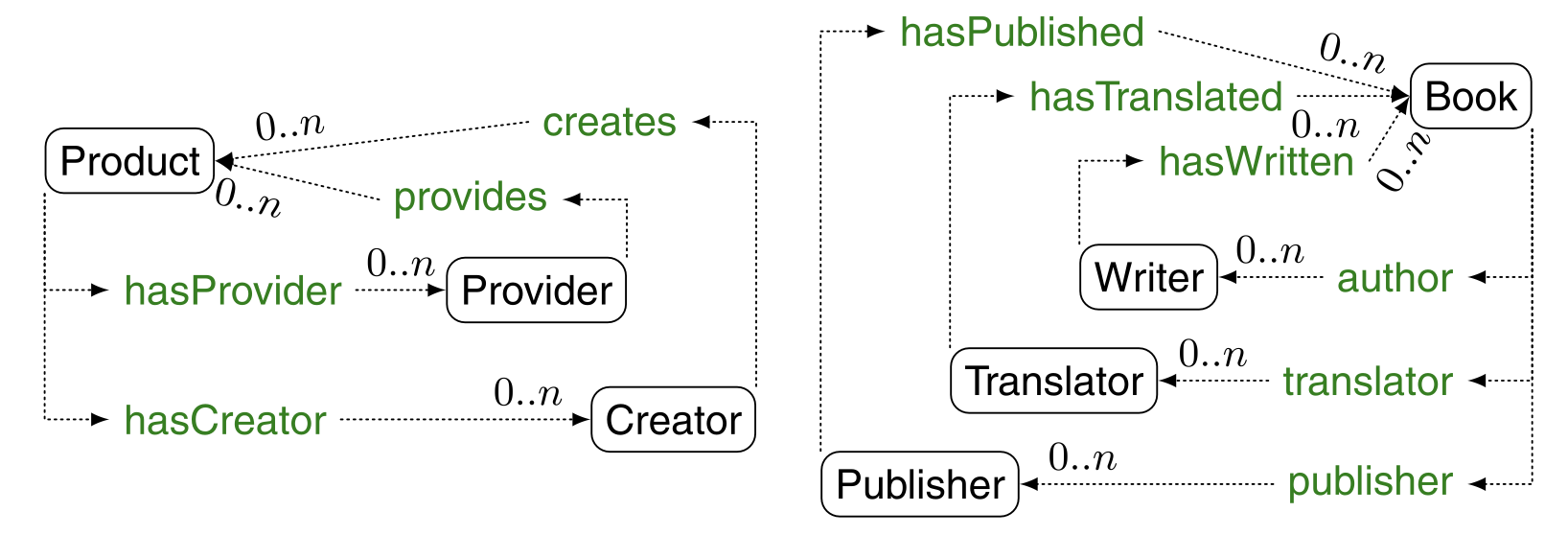
The computation of composite similarity is still local, since it only considers the neighbors of the nodes to provide the similarity. However, the similarity is for the entire ontology, and the final similarity value may ultimately depend on all ontology entities. Furthermore, if the ontology is not reduced to a directed acyclic graph, distances defined in a local way may be defined in a circular way. This is the most common case. For example, it occurs when the distance between two classes depends on the distance between instances that depend on the distance between the classes, or when there is a circulation in the ontology. As shown in the figure below, the similarity between Product and Book depends on the similarity between hasProvider and hasCreator and author, publisher, and translator. And the similarity between these elements ultimately depends on the similarity between Product and Book. These two graphs are homo-morphic in many ways.

Two typical ontologies with reference cycles: how do we match them?
In the presence of cyclic dependency, it is not possible to compute similarity locally. The classical way to deal with such a problem would be to iteratively calculate the distance or similarity, improving the last calculated value at each step. This is illustrated in the figure below.

Iterative calculation of fixed points of similarity and distance functions
For such a case, we need to define a strategy to compute this global similarity. Here we present two such methods: the first is defined as a process of propagating similarity in a graph, and the second transforms the definition of similarity into a set of equations, which are then solved by numerical techniques.
Similarity Flooding
Similarity Flooding (Melnik et al. 2002) is a popular graph matching algorithm that uses fixed-point computation to determine the corresponding nodes in a graph. This algorithm has been implemented in the Rondo environment.
The principle of this algorithm becomes that the similarity between two nodes must depend on the similarity between neighboring nodes (whatever the relation to be considered). The algorithm to achieve this is as follows.
- Transform the ontology into a directed labeled (multi) graph G: In this graph, a node is a pair of ontology concepts, and an edge exists between two nodes if there is a relationship between both ontologies in the two pairs of nodes. For example, in the ontology below, ⟨Provider, Writer⟩ is related to ⟨Product, Book⟩ and ⟨hasProvider, hasWritten⟩ are related via the edges labeled ⟨hasProvider, hasWritten⟩. In fact, the original Similarity flooding algorithm only connects nodes whose edges have the same label. This graph is closed by symmetry, which means that there are also edges in the opposite direction.

- Weight the edges: The weight is usually 1/n, which is equal to the outlierness (number of outgoing edges) of the source node. The description of the algorithm does not say what to do if several edges with different labels link pairs of the same concept, or if there are already edges in the opposite direction. The idea is to aggregate the weights in a triangular norm.
- Assign an initial similarity σ0 to each node: (Use the basic method for labels, or use a uniform assignment of 1.0.
- Calculate σi+1 for each node with the selected formula.
- Normalize all σi+1 obtained by dividing by the maximum value.
- If none of the similarities change above a certain threshold ε, i.e., ∀e ∈ o, e′ ∈ o′, |σ i+1(e, e′)
o′, |σ i+1(e, e′) – σ i (e, e′)| < ε, or after a given number of steps, stop, otherwise go to step 4.
The aggregation function chosen is a weighted linear aggregation, where the edge weights are the reciprocal of the number of other edges with the same label that reach the same pair of entities. The weights of the edges will be the reciprocal of the number of other edges with the same label that reach the same pair of entities.
[ sigma^{i+1}(x,x’)=sigma^0(x,x’)+displaystyle sum_{<<y,y’>,p,<x,x’>in G}sigma^i(y,y’)timesomega(<<y,y’>,p,<x,x’>>)]Variations of this equation have been considered, such as suppressing the σ0 term and replacing σ0 with σi, or using σ0(x,x′)+σi(x,x′) as the recurrence term. The former speeds up the computation, while the latter places importance on the initial values.
The convergence of this algorithm is not clear. (Melnik et al. 2005) provides the conditions under which the algorithm converges. The algorithm needs to provide a measure of similarity from which an alignment can be extracted.
Starting with the similarity flooding example, the ontology below, we will assume that all properties have the same name since the similarity flooding algorithm works with the same property name and there are no similar properties. From these ontologies, we generate the following labeled directed graphs (with weights).

The initial dissimilarities will be those provided in the weighted sum with weights of 1/4 and 3/4.
 The first iteration of the Similarity flooding algorithm to compute σ1 is shown below (left is the value of σi, right is the normalized result).

If we continue the iterative production and set e=0.1, we get the following result at the 17th iteration.

From these similarity values, we can extract the expected correspondences.
The following correspondences can be expected: dence Product = Book, Publisher = Provider, Writer = Creator.
Fixed points of similarity equations
OLA (Sect. 8.3.8) (Euzenat and Valtchev 2004) provides a way to deal with circularity and dependencies between similarity definitions.
In this case, the similarity value is represented as a set of equations where each variable corresponds to the similarity between a pair of nodes. There are the same number of equations as variables. The structure of each equation follows the definition of the respective similarity function for the underlying node category.
Given two classes c and c′, the resulting similarity function for the class is as follows
begin{eqnarray} sigma`C(c,c’)&=&pi_L^Csigma_L(lambda(c),lambda(c’)\&=&pi_O^CMSim_O(L(c),L'(c’))\&=&pi_S^CMSim_C(S(c),S'(c’))\&=&pi_P^CMSim_P(A(c),A'(c’)) end{eqnarray}
λ(⋅) L(⋅), S(⋅), and A(⋅) are functions that return class labels, instances, superclasses, subclasses, and properties, respectively (equivalent to name, properties, direct subclasses, direct superclasses, and direct MSim-measure is the similarity between a set of ontology entities and is described below. (pi_F^C) will be the weights that indicate the relative importance of feature F.
This function is normalized because the sum of the weights is equal to one. That is, (pi_L^C+pi_S^C+pi_O^C+pi_P^C=1), whereas each element spanning a collection of nodes or feature values is averaged with the size of the largest collection.
If each similarity expression is a linear aggregation of other similarity variables, then the system can be solved directly since all variables are degree1. However, in the case of OWL and many other languages, the system is not linear and there may be many candidate pairs for the best match. Similarity may depend on matching multiple edges that have similar labels output from the target node. In this approach, the similarity is computed by the MSim function, which first finds the alignment between the set of entities under consideration and then computes the aggregated similarity with respect to this matching.
In this respect, the OLA algorithm solves a very special problem: the maximum weight graph matching problem with weights that depend on the matching.
Nevertheless, the solution of the resulting system can be carried out as an iterative process that simulates the computation of the maximum fixed point of a vector function, as shown in (Bisson 1992). This point consists of defining an approximation of the MSim-measures, solving the system, replacing the approximation with a newly computed solution, and iterating. The first value of these MSim-measures is the maximum similarity obtained for one pair, without considering the dependent part of the equation. The subsequent values are the values of the full similarity equation satisfied by the system’s solution. Local matching varies from one step to another, depending on the value of the similarity.
However, the system converges because the similarity can only increase (the invariant part of the equation remains, and all dependencies are positive), and the similarity is bounded by a value of 1 or so. If the last iteration does not yield a gain greater than a certain ε value, the iteration stops. Even if the algorithm converges, it may stop at a local optimum. (That is, finding another match in MSim-measures does not increase the similarity value.) This could be improved by randomly changing these matches when the algorithm stops.
There are a few facts worth mentioning here. First, if there is no valid cyclic dependence between the similarity values, there is no need for different representations of the similarity function. The computational mechanism described above establishes the correct similarity values even if the order of the variables is appropriate. (The ordering implicitly follows a stepwise mechanism.) Moreover, if some similarity values (or similarity or (dissimilarity) claims) are obtained a priori, the corresponding expression can be replaced by that claim or value.
Example of the OLA algorithm. Since the problem to be solved is the same as the one defined in the Similarity Flooding example, the similarity of labels between classes will also be the same. The similarity of labels between properties is set to 1. (all are similar) for each pair of properties. Therefore, the initial similarity will be as follows

Equate the weights of the labels and properties for the classes ((pi_L^C=pi_P^C=1/2)) and the weights of the labels, ranges, and domains for the properties ((pi_L^P=pi_R^P=pi_D^P=1/3)). For the initial similarity (based on labels only), we obtain the following values
In the first iteration, the relationships between the entities are taken into account and the following results are obtained.
 After 3 iterations, the value does not change by more than e=0.1, and after 10 iterations, the value does not change by more than e=0.01, yielding the following results

For either epsilon value, the best match will always be the same. It is
For the class in the Similarity Flooding example, it looks like this, and for the properties, Creates = hasWritten, provides = hasPublished, hasProvided = publisher, hasCreated = author.
There are several similarities between the two methods. Both methods iterate through a set of equations extracted from the graphical form of the ontology. Both methods ultimately rely on computing proximities between undescribed language elements, such as data type names, values, URIs, and property type names. These proximities are propagated throughout the graph structure by similarity dependencies.
Furthermore, similarity flooding depends heavily on the identity of edge labels, whereas the OLA algorithm takes into account the similarity between properties. Furthermore, the OLA algorithm considers local mappings between alternative matching edges, rather than averaging over all possible matching edges. In other words, the OLA algorithm identifies matching subclasses and tries to propagate their similarity, while Similarity flooding propagates the average similarity of all pairs of subclasses, which is lower than the average similarity of all pairs of matching subclasses. Finally, convergence of Similarity flooding has not been generally proven.
Summary of Global Similarity Computation
The complexity of ontologies requires the propagation of similarity values between ontologies in an iterative fashion. Depending on what the definition of complex similarity is, and along what connections the links are propagated, there may be different propagation methods. As can be seen from the last technique, the computation of global similarity can be viewed as an optimization problem. Therefore, it is natural to consider classical optimization algorithms to achieve them.
In the next article, I will discuss two optimization methods: expectation maximization and particle swarm optimization.

コメント