Strategies in similarity matching methods (4) Learning to sort alignments
In the previous article, we discussed context-based matching, which is one of the ontology matching strategies. In this article, we will discuss another approach, weighted selection.
In this section, we describe an algorithm that learns how to sort alignments by presenting a number of correct alignments (positive examples) and incorrect alignments (negative examples). The main difference between these approaches is that the techniques in this section require some sample data for learning. This can be provided by the algorithm itself, such as only a subset of the correspondences to be judged, or it can be determined by the user, or it can be brought from external resources.

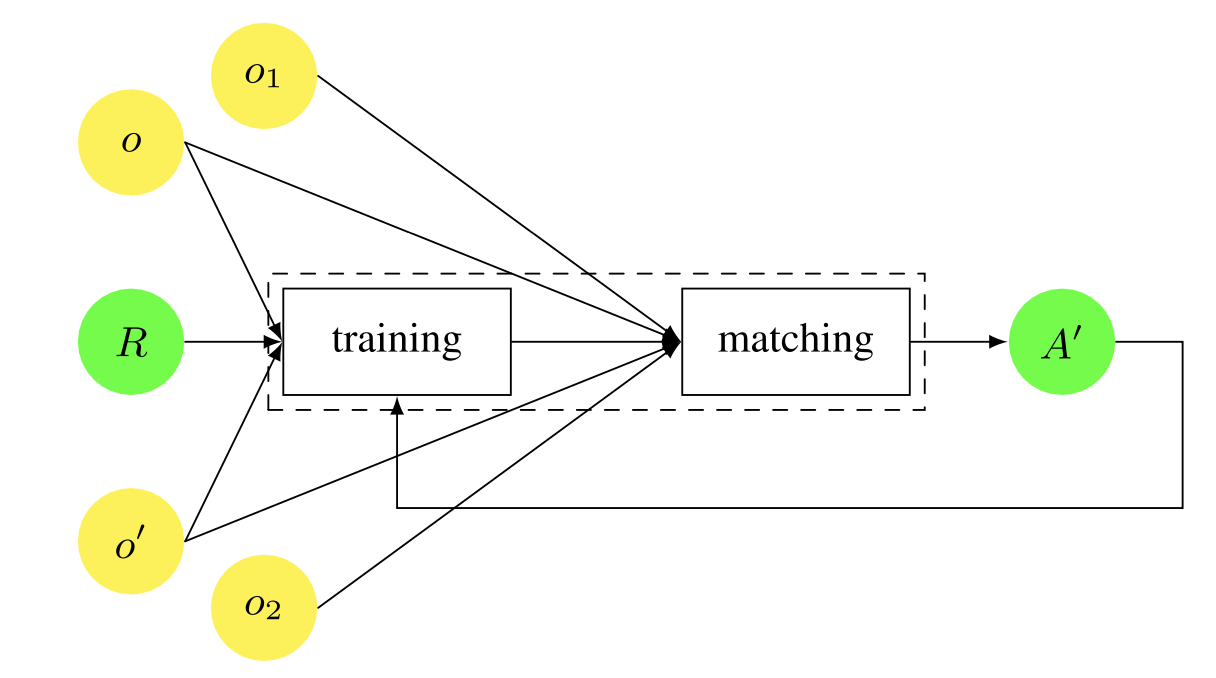
A typical machine learning setup for ontology matching. In supervised machine learning, from a limited reference (R) of the alignment to be obtained, the machine learning process generates an internal classification model, which is used to match the remaining fragments of o and o′, or new ontologies o1 and o2 with properties similar to o and o′. In unsupervised machine learning, the resulting alignment (A′) is usually injected as input to the training and iterated until certain conditions are met.
Matchers using machine learning usually operate in two phases. (1) a learning or training phase, and (2) a classification or matching phase. In the first phase, training data for the learning process is created, for example by manually matching two ontologies, and the system learns the matcher from this data. In the second stage, the learned matcher is used for matching new ontologies. Feedback on the obtained alignments is provided, which may be reflected again in step (1). Learning can be handled online so that the system can learn continuously, or offline if speed is more important than accuracy.
Usually, this process is done by dividing the data set (the set of positive and negative examples of alignment) into a training set (usually 80% of the data) and a control set (usually 20% of the data) that is used to evaluate the performance of the learning algorithm.
There are many types of information available to the learner. For example, it can be the frequency, format, location, and value distribution properties of words. In addition, multi-strategy learning methods can be effective when multiple learners are used to deal with patterns that each learner is good at. Finally, the results generated by various learners can be combined with the help of a meta-learner (Doan et al. 2003).
In this section, we discuss some of the well-known machine learning methods that have been used for text classification, such as Bayesian learning, WHIRL learning, neural networks, support vector machines, and decision trees.
Bayesian Learning
Naive Bayesian learning (Good 1965) is a probabilistic induction algorithm. It has been used as a classifier in various matching approaches (Doan et al. 2004, Straccia and Troncy 2006, Lambrix and Tan 2006, Nandi and Bernstein 2009, Spiliopoulos et al. 2010, Esposito et al. 2010, Tournaire et al. 2011).
Let the attribute x of one ontology be the attribute of another ontology (y1, . , ym, i = 1, …, m) of another ontology. , m) of another ontology (yi). In this approach, we consider the values of the attributes as a set of tokens, where V represents the basic set of values for attribute x. V = {t1,… ,tn}, where tj is the j-th token and j = 1,… ,n. Tokens are obtained by applying normalization techniques, such as lemmatization, to the words in the data instance; let P (yi ) be the probability that x matches yi a priori, i.e., without ever having seen a token of x. Next, let P (V ) denote the probability of observing the value V in x. Finally, let P (V |yi ) denote the conditional probability of observing the value V , given that x matches yi . Given a training example, Bayes’ theorem shows how to best predict the attributes of a data instance that has not been seen before. The attribute chosen will be the one that maximizes the posterior probability that x will match yi after seeing the value V . This is denoted by P (yi |V ) and is computed as follows
\[P(y_i|V)=\frac{P(V|y_i)\times P(y_i)}{P(V)}\]
This is called the Bayes rule. Naive Bayesian classifiers have a naive assumption that given yi, the tokens tj appear in V independently of each other. Based on this assumption, the parameters (tokens) of each attribute can be learned separately, which makes the learning process much simpler. Thus, if the attributes are class-independent, P(V|yi) can be decomposed into the product of P(t1|yi)×–P(tn|yi), and P(V ) can naturally be omitted from the Bayes rule. Thereafter, the Bayes rule can be rewritten as follows.
\[P(y_i|V)=P(y_i)\times \displaystyle\prod_{1\leq j \leq n}P(t_j|y_j)\]
The independence assumption often does not hold in practice. However, in many applications, violation of this assumption does not compromise the effectiveness of the approach (Domingos and Pazzani 1996).
The probabilities in the latter equation can be computed using training data; P(yi ) can be estimated as the fraction of examples matching yi , and P(tj|yi) can be estimated as k(tj,yi)/k(yi). where k(yi) is the total number of tokens in all training instances with attribute yi, and k(tj , yi ) is the number of occurrences of token tj in all training instances with attribute yi. Based on the above equation, the corresponding confidence score can be designed in an obvious way.
An example of training for naive Bayesian learning. Suppose we manually check that the attributes creator and name of one ontology match the attributes author and title of another ontology, respectively. This process consists of two steps.
The learning phase, in which we assume that Bertrand Russell is an instance of the creator attribute and My life is an instance of the name attribute. Therefore, based on this information, the following training examples can be given to the classifier: ⟨{‘Bertrand’, ‘Russell’}, author⟩ and ⟨{‘My’, ‘life’},title ⟩. The second declaration declares that {‘My’,’life’} is a title and that it has two tokens. The learner builds the internal classification model by examining the training instances. For example, if a word such as ‘life’ appears frequently in data instances related to the title and less frequently in data instances related to other fields, the learner realizes that its basic attributes are likely to match the title attributes and decides how to classify the data instances. If the training set is statistically representative, these frequencies can be converted to probabilities and Bayesian rules can be used. This can also be applied to classifying instances into classes, for example, ⟨{title:My title:life}, class:biography⟩.
Matching phase, where Life of Pi is an instance of the attribute h1 from the website structure that we want to match with the attributes of the second ontology above. The learner uses an internal classification model to predict the attributes and their confidence scores for a given instance. For example, ⟨author, 0.2⟩, ⟨title, 0.8⟩. Based on the confidence scores, we can conclude that h1 matches title.
WHIRL Learner
WHIRL is an extension of traditional relational databases that performs soft joins based on the similarity of text identifiers (not just based on equivalence of atomic values) (Cohen 1998) WHIRL has also been used for inductive classification of text, and it can be used in other The WHIRL approach to text classification can be regarded as a kind of nearest neighbor classification algorithm. That is, all training data is stored in memory and k instances are selected by Eu-clidean distance and used for (kNN) classification (Nottelmann and Straccia 2006; Spiliopoulos et al. 2010).
WHIRL has been used for matching to learn schema-level and instance-level information (Doan et al. 2003; Bilke and Naumann 2005). For example, ⟨location′,address⟩ says that if an entity in the ontology has the label location, it will match address. Extensions of the label′ can be obtained, for example, by including its synonyms, but the synonyms are obtained from coresponse tables manually created for the domain of interest WHIRL stores all the training examples it has seen. Assume we want to match another ontology o′ to ontology o. Given a label ′′ from o′, WHIRL computes the corresponding label of o based on the labels of all examples similar to label ′′ in the collection. This similarity is based on the TFIDF between the extended labels of the examples. For example, given a label phone for o′′ , WHIRL can generate a prediction as follows ⟨address, 0.1⟩, ⟨description, 0.2⟩, ⟨agent-phone, 0.7⟩. Based on the confidence scores, we can conclude that phone matches agent-phone.
In the case of instance-level information, this matcher uses the data tent instead of the expanded label. The training example in this case is of the form ⟨data instances′,label⟩, where data instances′ belong to ontology o′ and label belongs to ontology o. When matching a new ontology o′ to an ontology o, the TFIDF distance between any two examples is the distance between the data instances of o′ and the data instances of the WHIRL collection. Translated with www.DeepL.com/Translator (free version)
Neural Networks
An artificial neural network consists of nodes (or neurons) and weighted connections between them. The nodes are grouped into layers with inputs, outputs, and either none or one or more hidden layers. Usually, each node in the hidden layer is connected to all the nodes in the previous and next layers. Neural networks are widely used in practice because of their adaptability. Several types of neural networks have been used for various tasks in ontology matching. For example, they can discover correspondences between attributes through categorization and classification (Li and Clifton 1994, Esposito et al. 2010), learn matching parameters such as matcher weights to adjust the matching system for a particular matching task (Ehrig et al. 2005, Mao et al. 2010, Gracia et al. 2011). In this section, we focus on the first task described above, and the learning of matching parameters is discussed in a later section.
Given schema-level and instance-level information, it may be useful to classify this input into m categories in order to reduce the computational complexity of further manipulating the data. For this purpose, self-organizing map networks and corresponding self-organizing learning algorithms can be used (Koho-nen 2001). A self-organizing map network classifies n nodes in the input layer into m categories in the output layer. Usually, m is predefined based on how detailed the categories should be by setting the radius of the clusters. Input patterns and attributes (such as field length and data type) are considered as dimensions in the n-dimensional feature space. Neurons in the network are organized according to the characteristics of the given input pattern. This forms a clustered neuron structure, where neurons with similar characteristics are placed in related regions of the map. Each node in the output layer represents the center of the cluster.

In neural networks, matching is viewed as a classification problem. For this purpose, a backpropagation algorithm can be used. Backpropagation would be a supervision learning algorithm used to train the network to recognize input patterns and give them a corresponding score. First, the weights of the features are read into the input nodes, and then the weights are propagated forward to produce the output. If a misclassification is made, the error is propagated backwards to change the weights of the connections in the network. The weights are changed until the error in the output layer is no longer minimized.
Example 7.20 (Adapted from Neural Networks – (Li and Clifton 1994)) Given an ontology, attributes such as Employee.id, Dept.Employee, Payrol.SSN, etc. are close to each other in their input characteristics and propensity meaning, and can be clustered into one category Since their input characteristics and trend meanings are close to each other, they can be clustered into one category. The corresponding vector of cluster center weights is as follows ⟨0,0.1,0,…⟩ where the vector component represents the feature, the first position represents the data type, the second position represents the length, etc. An important feature for grouping the above mentioned attributes is the length of the field, because its value (0.1) is higher than the other values (0.0). In fact, the ID field is generally very regular (always use the full field), while the name field is more variable.
Figure 7.11 shows a three-layer network for recognizing patterns in m categories, given n features. The number of nodes in the hidden layer is arbitrary. Usually, it is chosen based on experiments to obtain the shortest learning time.
Learning phase. The training data for a neural network consists of a vector of cluster center weights and their target categories. For example, the previously mentioned vectors, i.e., ⟨0, 0.1, 0, 0, … … would look like this: ⟩ The vector ⟩ is tagged with the target category, number 3. The back propagation algorithm then adjusts the weights so that the properties of the at-tributes corresponding to these attributes make the output vector as close as possible to ⟨0, 0, 1, 0, …. The weights are adjusted so that the output vector is as close as possible to ⟩ The output vector is as close as possible to ⟨0, 0, 1, 0, …, indicating that the most likely category is 3. Translated with www.DeepL.com/Translator (free version)
Matching phase. In the matching phase, a new pattern of n features, e.g., the attribute health_Plan.Insured#, from another ontology o′ is input to the network trained with features from ontology o′. Based on the network’s internal classification model, determine the similarity between this pattern and each of the m categories. For example, this attribute matches category 3 (ID number) with a score of 0.92 and matches category 1 with a score of 0.05.
Support Vector Machine
Support Vector Machines (SVMs) can be a supervised learning method used for tasks such as classification and regression (Cristianini and Shawe-Taylor 2000). A basic SVM would be a non-probabilistic binary linear classifier. However, by using a kernel function, nonlinear classification can also be done efficiently. This implicitly transforms or maps the input of the SVM to a high-dimensional feature space, making data that were originally linearly non-separable easier to (possibly) separate in the feature space (Boser et al. 1992; Vapnik 2000). in several matching approaches (Ehrig et al. 2005; Spiliopoulos et al. 2010; Tournaire et al. 2011).
The training instances are divided into two categories, matched and unmatched, and the SVM constructs a maximum separation hyperplane in a high-dimensional space, i.e. (w,b), based on these. Here, w is the weight vector and b is the bias. The decision function is f (x) = w × x + b, where the margin or the distance between the closest data points is the maximum (this can be done software-wise, i.e. by considering noise and wrong examples (Cortes and Vapnik 1995)). The hyperplane decision function using the kernel is expressed as follows
\[ f(x)=w\times x+b=\displaystyle\sum_{i=1}^ny_i\alpha_iK(x_i,x)+b \]
n is the number of training examples, yi ∈ {+1, -1} is the congruent or incongruent label of example i, and K is the kernel function. αi is the Lagrange multiplier of each training point, where αi ≥ 0 and αi yi = 0. Only the training example (xi ) that is located close to the decision boundary, where αi > 0, and whose removal would change the solution, is called a support vector.
An example of a support vector machine. Given two ontologies, pairs of entities to be matched are extracted, such as ⟨name, title⟩ and ⟨id, isbn⟩. For each of these, feature selection is performed by similarity calculation using SMOA, n-gram, or WordNet. The end result of this operation can be seen as a similarity cube. Here, the first dimension represents the entities of the first ontology, the second dimension represents the entities of the second ontology, and the third dimension represents the applied features. For each entity pair, a target value, i.e. match or no-match label, is added. In the example above, both entities are matched. This is usually set by the domain expert when preparing the training data set. That is, they cut out vectors from the similarity cube and give them target values. These similarity vectors form a vector space, which is then trained to construct the maximum separation hyperplane. The quality of the final result will be determined by the choice of features and kernel types. Selecting the right kernel for the matching problem, i.e., a kernel that avoids irrelevant features, will improve the results. A variety of kernels can be used, such as polynomial kernels, Gaussian radial basis function kernels, string kernels, Bag of words kernels, etc. In the matching phase, the trained model is fed with new unknown features corresponding to pairs of entities and classified as match or mismatch by SVM.
Decision Trees
A decision tree classifier can learn a set of rules that are applied continuously and finally make a decision.
Traditional methods have the disadvantage that they are expressed in numerical values, which cannot be easily interpreted by humans, but decision trees do not have this disadvantage. A divide-and-conquer strategy can be used to learn a decision tree for a certain category. With them, in a training set T of features and instances characterized by the category, the feature f1 that best identifies the population (with respect to the set of categories) is selected. Then, when T is divided into two subsets, the subset T yes corresponding to the feature f1 and the subset no 1 yes no T1 which does not have this feature.
This procedure is applied recursively to T1 and T1. It stops when all instances in a subset are assigned to the same category. The decision tree learner generates a tree of rules whose leaves are the assignments to the actual categories. The decision tree learner can tolerate and accept that some of the instances are misclassified, as long as the tree can be greatly simplified. This can be useful when there are errors in the training set.
Decision trees can be used in ontology matching to discover correspondences between entities (Xu and Embley 2003; Duchateau et al. 2009; Spiliopoulos et al. 2010; Tournaire et al. 2011) and to match a given matching task with (Xu and Embley 2003; Duchateau et al. 2009; Spiliopoulos et al. 2010; Tournaire et al. 2011), and learning matching system parameters (e.g., thresholds) to automatically adapt to a given matching task (Ehrig et al. 2005; Duchateau et al. 2008). In this section, we focus on the former, and the learning of matching parameters is discussed in a later section.
Example of a decision tree. Given a large training alignment between instances from the two ontologies in the figure below, we apply decision tree learning, e.g. the C4.5 decision tree induction system (Quinlan 1993), to generate rules for identifying new instances.

The figure below shows a fragment of a decision tree that can be learned. The decision first shows that only matching of books from the first ontology to the second ontology is possible. Next, it distinguishes between books whose authors have one professor and books whose authors do not have a professor. We can then consider that if the author is the topic of the book, the book should be classified as an autobiography, otherwise it should be classified as an essay.
The decision tree is built with a certain amount of tolerance. The number after the targhetto category indicates the number of correctly and incorrectly recognized instances in the training set.
A fragment of a binary decision tree. Each node has a condition attached to it that must be satisfied by the item to be classified. If no further classification is possible, the resulting target category is shown, along with the number of correctly and incorrectly classified items in the training set (in parentheses).
The decision tree in the figure above can be rewritten as a mapping from the source ontology to the target ontology; the mapping rule corresponding to the Autobiography branch can be written as follows
Book(e) ∧ ∃e′; author(e, e′) ∧ Professor(e′) ∧ ∃e′; author(e, e′) ∧ topic(e, e′)
⇒ Autobiography(e)
Such rules can be translated into correspondences, albeit in an expressive language. A similar approach can be used for learning from structures rather than instances. (Xu and Embley 2003) show how to use decision trees to learn rules for matching terms in WordNet.
Summary of Matcher Learning
In this section, we have discussed basic matcher learning, which is basically viewed as a classification problem. many of the methods presented, such as Naive Bayes, kNN, SVM, and C4.5, are built on top of the data mining software Weka3 (Witten et al. 2011) for matching They have been used. A few specific frameworks, such as Neu-roph4 for neural networks and libSVM5 for support vector machines, have also been used successfully for matching purposes. These methods, their variants, and other learning techniques have been compared in detail in GLUE, CSR, and YAM++ matching approaches.
Technically speaking, preparing a training and test dataset and directly executing the methods in the above packages rarely yields good results right away. In many cases, issues such as overfitting and proper method parameter selection need to be addressed in order to obtain acceptable results. On the application side, machine learning approaches are useful in data integration scenarios that usually occur in vertical domains (see Section 1.2), where new ontologies have to be matched against a pool of existing ontologies. Therefore, previously learned matchers can be easily reused.
In the next article, we will discuss the tuning of ontology matching.

コメント