Artificial Intelligence Technology Web Technology Knowledge Information Processing Technology Semantic Web Technology Ontology Technology Natural Language Processing Machine learning Ontology Matching Technology
Continuing from the previous article on ontology matching. In the previous article, we discussed machine learning for alignment sorting. In this article, we will discuss the tuning approach for matching.
Tuning
Tuning is the process of improving the functionality of the matcher by adjusting it from the following perspectives.
- Improving the quality of the matching results (measured by accuracy, recalls, F-values, etc.).
- Improving the performance of the matcher, as measured by execution time and resource consumption such as main memory, CPU, and bandwidth.

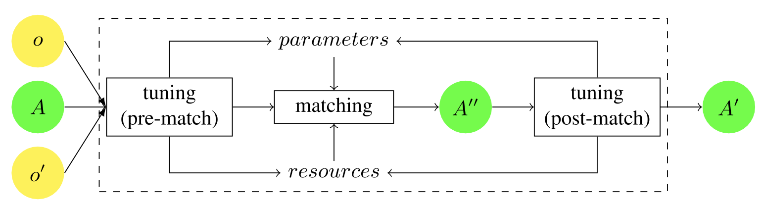
General framework for tuning. Before matching, tuning pre-determines which matcher to employ, for example, based on certain properties of the input ontology. After matching, the output alignment (A′′) of the matcher is evaluated by the tuner, and the parameters (and optionally the resources) of the matcher can be adjusted. The matcher then generates a new alignment with the adapted parameters. This process is repeated until the tuner can no longer provide better parameters, and finally returns the computed alignment (A′).
The tuning is usually done before matching, i.e., as a pre-match effort, after matching, i.e., as a post-match effort, or iteratively, i.e., involving both or one of the two aforementioned stages. This adjustment process can be done automatically, semi-automatically, or manually. The user makes adjustments before or after matching, either by using a graphic interface or by directly editing a configuration file. For example, before matching, the input ontology can be analyzed (manually or automatically) to gain actionable insights, such as whether the labels are long or short, how well developed the structure is, and whether there are instances or not. This information can be used to dynamically decide in advance (based on the input) whether to apply or not a particular matcher, such as a structure-level matcher, to the default matching workflow. On the other hand, the selection of matchers is often operationally handled by setting appropriate weights ([0 1]) for the matchers to be included in a predefined pool (usually at most a few dozen matchers) and further aggregated. So far, most design-time toolboxes have manually selected the weights (Do and Rahm 2007; Gal and Shvaiko 2009). Tuning is often done using pre-defined rules (Mochol and Jentzsch 2008; Li et al. 2009; Peukert et al. 2009) In implementations, tuning and matching are tightly coupled, and tuning may appear to be a runtime activity In some implementations (e.g., Mochol and Jentzsch 2008; Li et al. 2009; Peukert et al.
From a methodological point of view, tuning can be applied at different levels of architectural granularity. For example, a specific matcher, such as edit distance, can be selected from a library of matchers, and the parameters of the selected matcher can be set. For example, weighting, applying constraints such as 1:1 alignment, and selecting the final alignment. In these examples, an informed decision needs to be made to select a specific threshold, for example, 0.55, 0.57, or 0.6. If the tool provides a library of matchers, it may be difficult for the user to select, configure, and parameterize the matchers because the solution space is too large to try all the options. Therefore, efforts are being made to make this happen automatically. This is sometimes referred to as ontology meta-matching (Lee et al. 2007; Eckert et al. 2009). In practice, since these operations are always performed within a predefined number of alternatives and can often be reduced to a (sophisticated) variant of parameter tuning, we will consider the above operations together.
As the definition of the matching process indicates, a matcher can use an input alignment A, a parameter p (such as a weight), and an external resource r, in addition to the two input ontologies. These three elements make up the tunable matcher configuration cfg = {⟨A, p, r⟩}. For simplicity, these three elements can be generalized and represented as a set of pairs as follows.
\[cfg = \{⟨p_1,v_1⟩,\dots,⟨p_n,v_n⟩\}\]
The parameter (pi) and its value (vi) in the above equation, e.g., the threshold value is 0.55, and the CFG is the space of all possible configurations. The goal of tuning will be to find the optimal configuration, i.e., one where changing the parameters does not degrade the quality of matching (e.g., accuracy), the performance of the matcher (e.g., execution time), or both. For example, optimizing the matching quality by F-measure means finding a cfg∗ in the CFG space that improves F-measure.
Use Cases
eTuner takes a design-time tuning approach to its library of schema matchers. Given a specific matching task, it automatically adjusts the matching system by selecting the appropriate matcher and the best parameters to use, such as thresholds. eTuner uses decision trees as aggragation functions, where nodes represent similarity measures and edges are used as conditions on the result. MatchPlanner uses a decision tree as an aggregration function, where nodes represent similarity measures and edges are used as conditions on the result. Such a decision tree represents a plan with the matching algorithm as the basic operation. Furthermore, since the edges of the decision tree are used as conditions, these can be regarded as thresholds tailored to each matcher. ECOMatch (Ritze and Paulheim 2011), on the other hand, uses a user-supplied alignment sample and optimizes a partial F-measure on this sample. ECOMatch views the matcher as a black box and uses out-of-the-box optimization ECOMatch sees the eliminator as a black box and uses out-of-the-box optimization techniques to find the optimal parameters for these systems. This allows us to select both the best matcher and parameters. AMS uses a rule-based approach to adapt the matching process. Both input and output properties are considered as properties accessible to the rules. Rules are invoked in specific contexts to modify the workflow. For example, they add aggregators (when there is more than one result) or suppress basic matchers (when the quality is not good enough).
In the following, two specific methods for aggregating and tuning basic matchers will be explained in detail with examples. These are stacked generalization and genetic algorithm.
Stacked Generalization
Stacked generalization is an approach that combines multiple learning algorithms (Wolpert 1992). In terms of ontology matching, this approach can aggregate multiple basic learners, such as Naive Bayes and WHIRL, for a particular label (Doan et al. 2003; Esposito et al. 2010).
The learning phase of stacked generalization consists of two steps. In the first step, the output of each learner is collected to create a new data set. First, let D0 = {⟨ci , xi ⟩}i=1,…,m be the training dataset. ,m be the training dataset, where ci is a category and xi is an instance represented by a vector of features. In terms of ontology matching, ci is an entity of ontology o, and xi is an entity of ontology o′. Here, for example, an individual ci represented by its attributes is the category to which xi should be assigned, and in the case of ontology matching, it is the entity corresponding to xi. In order to avoid over-fitting, we will now perform cross-validation to ensure that the training data contains the query instances. Specifically, D0 is randomly partitioned into p most equal parts, (D_1^0, dots, D_p^0), where (D_k^0) is the test and (overline{D}_k^0 = D^0 – D_k^0) is the training set for the kth class of cross-validation. Given q basic learning algorithms (matchers), called level 0 generalizers, using the lth matching algorithm for the training set (overline{D}_k) yields the learned model (M_l^k). Such a model, given a vector of features characterizing an object, returns a prediction which is the category to which the object should be assigned. This will be the level 0 model; let (M_l^i) be the prediction of model (M_l^k) for xi∈Dk. The end result of cross-validation is a set D1 consisting of exactly one prediction for each of the training examples.
\[D^1=\{<c_i,<M_1^i,\dots,M_q^i>>\}_{i=1,\dots,m}\]
The output of the first stage is used as input data for the second stage, where another learning algorithm called the level-1 generalist is employed. The level-1 generalizer then derives a level-1 model M’ for (M_1^i , dots, M_q^i) for ci. Thus, while the level-0 classifier deals with the possibility of assigning an entity to a category with respect to its attributes, the level-1 classifier deals with the possibility of assigning the same entity to the same category with respect to the category predicted by the classifier.
In the classification phase, given a new instance x, the learned model generates vectors ⟨M1, … , Mq>. This will be the input to M′ , and M′ will output the final classification of that instance.
(Ting and Witten 1999) found that, compared to learning algorithms such as C4.5 decision trees (Section 7.5.5) and Naive Bayes (Section 7.5.1), (1) the higher-level model combines confidence rather than prediction of the lower-level model, and (2) multi-reactive linear regression is used as a level-1 generalizer. We confirm that the best results are obtained with stack generalization for the classification task when it is used.
In addition to multi-response linear regression, there are other algorithms that work equally well for this task, such as neural networks.
An example of stacked generalization. (Adapted from (Doan et al. 2003)) Assume we use two basic types of learners. These will be (1) the WHIRL learner, which deals with labels of entities, and (2) the Naive Bayesian learner, which deals with data instances of entities. In this example, we abbreviate the names of these matchers as WHIRL and NB, respectively.
Training Phase Consider the label address from ontology o.
The table below shows an example of relevant training data for the basic learner from ontology o′.
Columns 1 and 2 contain the labels (e.g., location) of some entities in the ontology o′ and the underlying data instances (e.g., ⟨Miami, FL⟩). columns 4 and 5 contain the labels of the WHIRL and Naive Bayes describe the confidence score S generated by cross-validation based on the inputs from the first three columns.
For example, Saddress(location) = 0.5 and Saddress(⟨Miami, FL⟩) = 0.8. Finally, the WHIRL NB
The last column indicates whether the target correspondence is valid or not. For example, the location from o′ actually matches the address from o, so the corresponding value in the last column is 1. On the other hand, the displayed price does not match the address, so the corresponding value in the last column is 0.
The information in the three rightmost columns will be used as input for the linear regression.
used as input for ear regression (Breiman 1996; Birkes and Dodge 2001). the results of WHIRL and the naïve Bayesian learner represent the confidence score (S), and the last column represents the value of the response variable.
column represents the value of the response variable. As a result of least squares minimization, the weight assigned to the pair of WHIRL and label address is 0.2. This means that Waddress = 0.2 and Waddress = 0.9. Interpreting the weights of this WHIRL NB, it seems that based on the accumulated generalization training, the naive Bayesian learner is much more reliable than WHIRL in predicting about the advertisement dress.

Matching phase WHIRL analyzes the label area and generates a confidence score (e.g., ⟨address,0.4⟩). On the other hand, the naive Bayesian learner analyzes the content of the data and generates a confidence score (e.g., ⟨address,0.8⟩). Using the weights obtained in the training phase of stacked generalization, the weighted average of the confidence scores can be calculated as follows: 0.4 × 0.2 + 0.8 × 0.9 = 0.8, yielding the integrated prediction ⟨address, 0.8⟩.
There are other methods with similar goals, such as Boosting and Bagging. To combine the judgments of individual models (matchers), Boosting uses weighted majority voting and Bagging uses unweighted majority voting. However, these require a large number of models because they rely on varying the data distribution to obtain a diverse set of models from a single learning algorithm, while stacking can work with only a small number of level-0 models (Ting and Witten 1999). SMB systems are considering using boosting (with the AdaBoost algorithm) to select matchers from a pool for further combination.
Genetic Algorithm
The genetic algorithm is a population-based computational model inspired by genetics and evolution (Holland 1992). It is an adaptive heuristic search method that is often used for complex parameter optimization problems. Genetic algorithms essentially perform a randomized global search in the solution space (Mitchell 1996).
Individuals in the population are considered as solutions, and the environment in which they live corresponds to the objectives and constraints of the problem to which these individuals are adapted. In the selection process, the principle of survival of the fittest is applied. Through the generations of the population, called iterations, the preferred attributes of the individuals (promising solutions) are pushed forward in the evolutionary process, and weak solutions are driven out of the population. The main components of a genetic algorithm will be as follows.
Encoding The original problem space is known as the phenotype space, which is encoded into the genetic space, the genotype space, for the search. Before the result can be produced, the genotype must be decoded into the phenotype space. Individuals are represented as data structures like genotypes in a population, as binary, integer, or real strings. Each string element represents a specific characteristic of the solution.
Initialization of the Population The initial population is initialized by randomly generating, say, 1000 individuals, but problem-specific heuristics can also be used, thereby improving the goodness of fit of the initial individuals.
Evaluation Each individual in the population is evaluated using a fitness function to determine its quality and to determine its respective reproductive opportunities, i.e., which important information to preserve and pass on to its offspring. This will result in 1000 individuals being ranked down based on the value of the fitness function.
Parental Selection Parental selection is used to select the parents for offspring. For example, there is a method called roulette wheel sampling, which selects individuals randomly with a probability proportional to their fitness. For example, of 1000 ordered individuals, the first half of the individuals can be selected as parents.
Crossover This would be a variance operation used to combine the genotypic characteristics of the two parents to create one or two offspring genotypes. It is often a stochastic operation.
Variation This would be another variation operation used to change the genotype of a parent to slightly alter its offspring. This will be a stochastic operation. This operation is motivated by the possibility of reinserting lost (intergenerational) information in order to prevent premature convergence without reaching a satisfactory solution and to promote genetic diversity.
Population generation New individuals are created by crossover and mutation, and the next generation is created. Individuals in the population are evaluated for their fitness.
Termination Conditions Appropriate termination conditions need to be determined. For example, when the fitness level reaches the desired accuracy, or when the fitness does not improve after a certain number of iterations. This is usually handled by a threshold value.
Genetic algorithms have been used in the context of ontology matching for a variety of purposes. For example, genetic algorithms have been used in (Vázquez-Naya et al. 2010) to search for the best combination of multiple matchers and aggregate their re- sults into a single value, and in (Wang et al. 2006) and (Elmeleegy et al. 2008) to extend type similarity and use type similarity have been used to determine the globally optimal alignment with respect to the similarity features that make up the fitness function. Finally, genetic algorithms have also been used as a near-optimal alignment extraction strategy (Section.7.7) for alignment selection (Qazvinian et al. 2008).
Example of Genetic Algorithm Consider the use of a genetic algorithm to optimally aggregate multiple matchers (Vázquez-Naya et al. 2010). The challenge is to discover weights that maximize the global alignment quality. Each individual represents a potential solution, i.e., a set of weights, the sum of which is 1. The decoding of genotypes is done in ascending order of the separation values. The process starts with a randomly generated aggregate, i.e., a set of weights for each. For example, the results of five different matchers must be aggregated, and the configuration of the i-th genotype could be the following four separation points: 0.51, 0.11, 0.92, 0.57, whose decoding (reordering) would be: 0.11, 0.51, 0.57, 0. The weights of the matchers are calculated as the difference of the separation points: w1 = 0.11, w2 = 0.40, w3 = 0.06, w4 = 0.35, w5 = 0.08. F-measure is used as the fitness function. The selection of parents is done by the roulette wheel method. Crossover passes only those offspring that exceed the fitness of the parents to the next generation. Mutation is done with low probability, replacing elements of the genotype with randomly generated ones. The best individuals from one generation are copied to the next. This process stops when the individual fitness function becomes higher than a threshold value. The most fit individual is decoded as the final selected solution.
Summary of Matcher Tuning
In this section, we have introduced a general framework for tuning and described two specific methods, including stacked generalization and genetic algorithms. These methods are used to make the matching system work better by aggregating the underlying matchers. This topic has emerged in recent years and requires further investigation. In practice, many different constraints and requirements apply to the matching task, such as correctness, completeness, execution time, main memory, etc., and multi-criteria decisions are required. The main challenge lies in semi-automatically combining matchers by looking for complementarities, balancing component weaknesses, and enhancing strengths. For example, aggregation is usually done according to a pre-defined aggregation function, such as a weighted average. Work on evaluation can be used to assess the strengths and weaknesses of individual matchers by comparing their results with the requirements of the task. New methods for performing the aggregation that can prove the quality of the alignment must be explored.
In the next article, we will discuss another approach to matching optimization, the alignment extraction approach.

コメント