Implementation of Neural Networks and Error Back Propagation using Clojure
With the introduction of small-scale deep learning in algorithms for reinforcement learning, online learning, etc. in mind, I describe the implementation of neural nets in Clojure (including an understanding of the principles of neural net algorithms). The base implementation is based on the article “Building a Neural Network from Zero and Observing Hidden Layers in Clojure” on qita, with some additions.
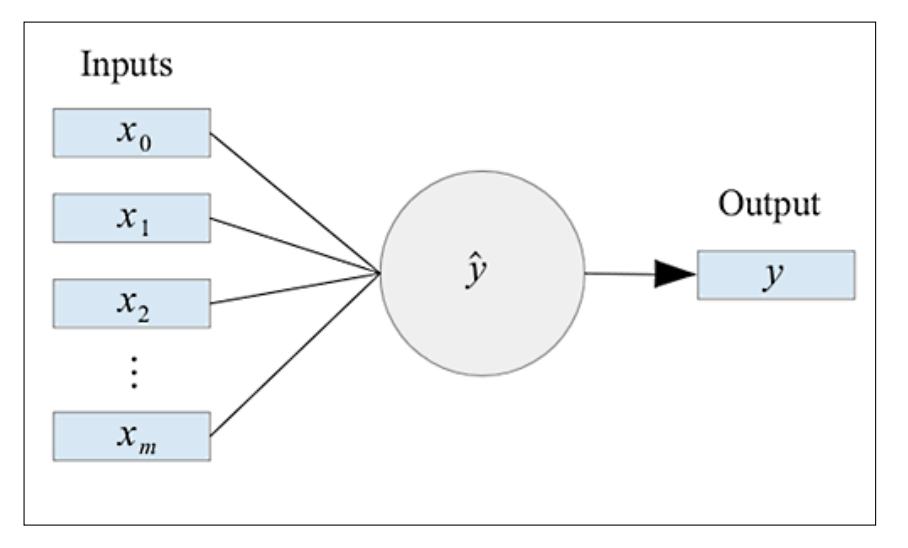
See “Getting Started with Clojure” for details on setting up the Clojure environment. Also, since the library uses incanter, it is necessary to add incanter to project.clj. A neural network is represented as follows.

The formula is expressed as follows
\[\hat{y}=g\left(\sum_{i=0}^mx_iw_i\right)\ where\ g(x,w)\ is\ the\ activation\ function\]
This can be translated into Clojure code as follows.
(defn unit-output [input-list w-list bias activate-fn-key]
  (let [activate-fn (condp = activate-fn-key
                      :sigmoid sigmoid
                      :linear  identity)]
    (->> (mapv * input-list w-list)   ;;(1)
         (cons bias)            ;;(2)
         (reduce +).                   ;;(3)
         activate-fn)))                ;;(4)
The inputs to the function are a list of input layers, a list of weights, and an activation function. The outputs are (1) the creation of an array of weights multiplied by the inputs, (2) the addition of a bias to the array, (3) addition, and (4) passing through the activation function for the final output.
The activation function is defined as follows. (in the case of a sigmoid function)

(defn sigmoid [x]
  (/ 1 (+ 1 (exp (- x)))))
Check the output.
(unit-output [1 2 3] [3 2 1] -2 :linear)   ;;8
(unit-output [1 2 3] [3 2 1] -2 :sigmoid)  ;;0.9996646498695336
(unit-output [1 2 3] [3 2 1] 1 :linear)    ;;11
(unit-output [2 4 -3] [-4 2 1] 1 :linear)    ;;-2
Next, consider the feed-forward multilayer perceptron.

Here, a neural net is expressed as follows.
[{:activate-fn :sigmoid :units [{:bias -2 :w-list [2]}
                                {:bias 1  :w-list [3]}
                                {:bias -3 :w-list [-4]}]}
 {:activate-fn :linear :units [{:bias -5 :w-list [1 -2 3]}]}]
The map data represented by {:activeta-fn …} represents one layer, and the :unit [{:bias -2 :w-list [2]}…] in it represents the weights or biases that a unit has.
Using these, the output of a unit on the network is represented as follows.
(defn network-output [w-network x-list]
  (loop [w-network w-network, input-list x-list, acc [x-list]]
    (if-let [layer (first w-network)]
      (let [{activate-fn :activate-fn units :units}  layer
            output-list (map (fn [{bias :bias w-list :w-list}]
                               (unit-output input-list w-list bias activate-fn))
                             units)]
        (recur (rest w-network) output-list (cons output-list acc)))
      (reverse acc))))
In the above code, the outer loop function performs the layer computation and the inner map function performs the computation for each unit in the layer, resulting in the total output of the unitary net.
Using these functions, a layer calculation with a scalar input [2], a sigmoid function as a hidden layer, and a linear function with a scalar output is performed as follows. (The result is the value of each of the three layers: input data, hidden layer, and output.)
(network-output
  [{:activate-fn :sigmoid :units [{:bias -2 :w-list [2]}
                                  {:bias 1  :w-list [3]}
                                  {:bias -3 :w-list [-4]}]}
   {:activate-fn :linear :units [{:bias -5 :w-list [1 -2 3]}]}]
  [2])

;;([2] (0.8807970779778823 0.9990889488055994 1.670142184809518E-5) (-6.117330715367772))
Learning with Neural Networks
The aforementioned results are used to compute the weights of the neural net. The weights can be calculated by means of pre-prepared input and output pairs. Basically, the framework is as supervised learning. Neural nets are trained using a method called error back propagation. The error back propagation method has two major processes.
- For each error between the result of the prediction and the correct answer, determine how much each unit is responsible for the error.
- By the amount of responsibility, each unit modifies its weights and biases.
This process is calculated in order from the output. First, for 1, the result of the forecast is subtracted from the political boundary, and since this is an error due to the output via the activation function, the derivative of the activation function is taken into account and the amount of responsibility of the unit at the output layer is calculated by multiplying the error and the derivative of the activation function by the unit’s output. This amount of responsibility is called the gradient and is expressed by the following equation
\[\Delta^{(l)}:=\Delta^{(l)}+\delta^{(l+1)}\left(a^{(l)}\right)^T\]
where a(l) is the activation value \(a^{(l)}=g\left(\Theta^{(l)}a^{(l-1)}\right)\), which is obtained by applying the activation function to the product of the weight matrix of one layer and the activation value of the previous layer. Also, δ(l) is the difference between the activation value a(l) and the expected output value.
For the second parameter, the amount of responsibility for the error (gradient) obtained in step 1 is used to update the parameters. To update a certain weight, two parameters other than the amount of responsibility are the magnitude of the lower-layer input subject to the weights and the learning rate, which are multiplied together and then updated from the original weights.
\[W^{(l)}:=W^{(l)}-\left(\rho\Delta^{(l)}+\Lambda\delta^{(l)}\right)\]
The Clojure code for error back propagation including the above is as follows.
(defn back-propagation [w-network training-x training-y learning-rate]
  (let [reversed-w-network (reverse w-network)
        reversed-output-net (reverse (network-output w-network training-x))]
    (loop [reversed-w-network reversed-w-network
           reversed-output-net reversed-output-net
           delta-list (mapv #(* (- %2 %1)
                               (derivative-value %2 (:activate-fn (first reversed-w-network))))
                           training-y (first reversed-output-net))
           acc []]
      (if-let [w-layer (first reversed-w-network)]
        (let [output-layer (first reversed-output-net)
              input-layer  (first (rest reversed-output-net))
              updated-w-list {:units (map (fn [{bias :bias w-list :w-list} delta]
                                            {:w-list (map (fn [w input]
                                                            (- w (* learning-rate delta input)))
                                                          w-list input-layer)
                                             :bias (- bias (* learning-rate delta))})
                                          (:units w-layer) delta-list)
                              :activate-fn (:activate-fn w-layer)}]
          (recur (rest reversed-w-network)
                 (rest reversed-output-net)
                 (map-indexed (fn [index unit-output]
                                (let [connected-w-list (map #(nth (:w-list %) index) (:units w-layer))]
                                  (* (->> (mapv #(* %1 %2) delta-list connected-w-list)
                                          (reduce +))
                                     (derivative-value unit-output (:activate-fn (first (rest reversed-w-network)))))))
                              input-layer)
                 (cons updated-w-list acc)))
        acc))))
The above code uses the training-x argument as the output of the input layer, training-y as the correct answer label, and loops to perform layer-by-layer calculations, with delta-list representing the amount of responsibility of each unit in that layer, and updated-w-list representing the weight and bias value of each unit updated in that layer.
updated-w-list represents the weight and bias value of each unit updated in that layer.
The connected-w-list represents the portion of the units in the upper layer that are connected to this unit in the middle layer.
The output of this function will also represent the information of a new neural net with updated weights and biases for all units.
The error back propagation is computed using these as follows.
(back-propagation
 [{:activate-fn :sigmoid :units [{:bias -2 :w-list [2]}
                                 {:bias 1 :w-list [3]}
                                 {:bias -3 :w-list [-4]}]}
  {:activate-fn :linear :units [{:bias -5 :w-list [1 -2 3]}]}]
 [2]
 [5]
 0.05)

=> ({:units ({:w-list (2.1167248411922994), :bias -1.9416375794038503}
             {:w-list (2.9979761540232905), :bias 0.9989880770116454}
             {:w-list (-3.9999442983612816), :bias -2.999972149180641}),
     :activate-fn :sigmoid}
    {:units ({:w-list (1.4896056204504848 -1.4446398871029504 3.000009283761505),
              :bias -4.444133464231611}),
     :activate-fn :linear})
We can see that the same form of weight network is output, with updated weights and bias values.
Initialization of neural nets
The method of initializing the weights of a neural net to compute learning by giving random numbers has become the mainstream method. The following is a simple code for initialization of a neural network with random numbers.
(defn init-w-network [network-info]
  (loop [network-info network-info, acc []]
    (if-let [layer-info (first (rest network-info))]
      (let [{n :unit-num a :activate-fn} layer-info
            {bottom-leyer-n :unit-num} (first network-info)]
        (recur (rest network-info)
               (cons {:activate-fn a
                      :units (repeatedly n (fn [] {:bias (rand) :w-list (repeatedly bottom-leyer-n rand)}))} acc)))
      (reverse acc))))
Using the above code, a feed-forward style net of 1=>3=>1 network is generated as follows.
(init-w-network [{:unit-num 1 :activate-fn :linear}
                 {:unit-num 3 :activate-fn :sigmoid}
                 {:unit-num 1 :activate-fn :linear}])

=> ({:activate-fn :sigmoid,
     :units ({:bias 0.7732887809599917, :w-list (0.9425957186019741)}
             {:bias 0.9502325742816429, :w-list (0.53860907921595)}
             {:bias 0.6318880361706507, :w-list (0.6481147062091354)})}
    {:activate-fn :linear,
     :units ({:bias 0.3295752168787115, :w-list (0.9050385230268984 0.5103400587715446 0.4064520926825912)})})
Learning on the entire data set
Iterate over the training data using the code so far.
(defn train [w-network training-list learning-rate]
  (loop  [w-network w-network, training-list training-list]
    (if-let [training (first training-list)]
      (recur (back-propagation w-network (:training-x training) (:training-y training) learning-rate) (rest training-list))
      w-network)))
The method of performing error back propagation on each piece of training data is called the stochastic gradient descent method. The gradient method itself is not limited to neural nets, but is a method used for optimization. There is also a method called “mini-batch,” which updates the data in batches after a certain degree of cohesion. The theoretical details of these methods are described in “Stochastic Optimization.
In addition, the error over the entire data set is calculated based on the sum of squared errors to evaluate whether the training is successful or not.
(defn sum-of-squares-error
  [w-network training-list]
  (loop [training-list training-list, acc 0]
    (let [{training-x :training-x training-y :training-y} (first training-list)]
      (if (and training-x training-y)
        (let [output-layer (first (reverse (network-output w-network training-x)))
              error (->> (mapv #(* 0.5 (- %1 %2) (- %1 %2)) output-layer training-y)
                         (reduce +))]
          (recur (rest training-list) (+ error acc)))
        acc))))
Finally, the condition for terminating the training is when the aforementioned error value becomes less than a certain value, and the function for training the neural network with these conditions is defined as follows. The theoretical consideration of the algorithm’s stopping condition is described in detail in “Continuous Optimization in Machine Learning“.
(defn training-loop [w-network training-list learning-rate epoc]
  (loop [w-network w-network, epoc epoc]
    (if (> epoc 0)
      (let [w-network (train w-network (shuffle training-list) learning-rate)
            error (sum-of-squares-error w-network training-list)]
        (println (str "epoc=> " epoc "nw-network=> " w-network "nerror=> " error"n"))
        (recur w-network  (dec epoc)))
      w-network)))
Application to Examples
Using the above, we will compute a concrete example.
Consider the following example of approximating them with a neural net using the following sin function as input.
(def training-list-sin3 (map (fn[x]{:training-x [x] :training-y [(sin x)]}) (range -3 3 0.2)))
The code for inference by a neural net with one input dimension and one output dimension in hidden layer 3 is as follows.
(let [hidden-num 3
      w-network (training-loop (init-w-network [{:unit-num 1 :activate-fn :linear}
                                                {:unit-num hidden-num :activate-fn :sigmoid}
                                                {:unit-num 1 :activate-fn :linear}]) training-list-sin3 0.05 10000)
      nn-plot (-> (function-plot sin -3 3)
                  (add-function #(first (last (network-output w-network [%]))) -3 3))]
  (loop [counter-list (range hidden-num), nn-plot nn-plot]
    (if-let [counter (first counter-list)]
      (let [nn-plot (-> nn-plot
                        (add-function #(nth (second (network-output w-network [%])) counter) -3 3)
                        (set-stroke-color java.awt.Color/gray :dataset (+ 2 counter)))]
        (recur (rest counter-list) nn-plot))
      (view nn-plot))))
The processing time is several tens of seconds and outputs the following results.

The red line is the correct data and the blue line is the result from the neural network. The gray line is the output result of the hidden layer.
General-purpose neural net tool
These are compiled as a DSK, and if the configuration parameters of the network and various optimization methods are entered as input, they are computed by Keras, which is described in the previous article “Deep Learning with Python and Keras: What is Deep Learning?
In Clojure, there are several similar libraries such as enclog, Neuroph, and FNN.
For example, enclog can be implemented in a very simple way as shown in the code below, and the computation speed is optimized for fast processing.
(ns clj-ml4.som
  (:use [enclog nnets training]))

(def som (network (neural-pattern :som) :input 4 :output 2))

(defn train-som [data]
  (let [trainer (trainer :basic-som :network som
                         :training-set data
                         :learning-rate 0.7
                         :neighborhood-fn (neighborhood-F :single))]
    (train trainer Double/NEGATIVE_INFINITY 10 [])))

(defn train-and-run-som []
  (let [input [[-1.0, -1.0, 1.0, 1.0 ]
               [1.0, 1.0, -1.0, -1.0]]
        input-data (data :basic-dataset input nil) ;no ideal data
        SOM        (train-som input-data)
        d1 (data :basic (first input))
        d2 (data :basic (second input))]
    (println "Pattern 1 class:" (.classify SOM d1))
    (println "Pattern 2 class:" (.classify SOM d2))
    SOM))

コメント