Artificial Intelligence Technology Web Technology Knowledge Information Processing Technology Semantic Web Technology Ontology Technology Natural Language Processing Machine learning Ontology Matching Technology
Continuing from the previous article on natural language similarity from ontology matching. In the previous article, we discussed an approach based on the internal structure of the data, such as its type and domain information. In this article, we will discuss an approach that extends these approaches further.
If two ontologies share the same set of indivisuals, matching becomes very easy. For example, if two classes share the exact same set of individuals, we can strongly presume that these classes are equivalent.
Even if the classes do not share the same set of individuals, the matching process can be based on tangible indicators that are not easily changed. For example, the title of a book has no reason to change. In other words, if a book has a different title, then it is not the same book. Then the matching would again be based on individual comparisons.
In this way, we can classify the extension methods into three categories: (1) those that apply to ontologies with a common instance set, (2) those that propose individual identification techniques before using conventional methods, and (3) those that do not require identification, i.e., those that apply to heterogeneous instance sets.
Comparing Common Extensions
The easiest way to compare classes that share instances would be to test the interrelationships between instance sets A and B and consider that these classes are very similar if A∩B =A=B and more general if A∩B =B or A∩B =A. Re-relationships and entity sets can be integrated mainly on the basis of aggregation relations.
- equal (A∩B =A=B), and
- Included (A∩B =A), Included (A∩B =A), Included (A∩B =B)
- Contained (A∩B =B), Separated (A∩B =∅)
- Separate (A∩B =∅)
- Duplicate
(Larson et al.) These challenges are responsiveness to faults. A small amount of erroneous data can cause the system to draw erroneous conclusions about the relationship between domains. Furthermore, the dissimilarity must be 1 if none of these cases apply. For example, a class may have some instances in common, but not all.
As a way to improve this, the Hamming distance between two extensions can be used. This corresponds to the magnitude of the symmetric difference normalized by the magnitude of the sum.
Definition 36 (Humming Distance)
The Humming distance between two sets is
a dissimilar function δ : 2E × 2E → R such that ∀x, y ⊆ E.
\[\delta(x,y)=\frac{|x\cup y-x\cap y|}{|x\cup y|}\]
This version of symmetric difference is normalized. Using such a distance to compare sets is more robust than using equality.
Similarity can also be calculated based on a probabilistic interpretation of a set of instances. This would be the case for Jaccard similarity (Jaccard 1901).
Definition 37 (Jaccard Similarity)
Given two sets A and B, where P (X) is
the probability of a random instance being included in set X,
Jaccard similarity is defined as
\[ \sigma(A,B)=\frac{P(A \cap B)}{P(A\cup B)} \]
This index is normalized and is 0 when A ∩ B = φ and 1 when A = B. This indicator can be used when two classes of different ontologies share the same set of instances.
Formal Concept Analysis
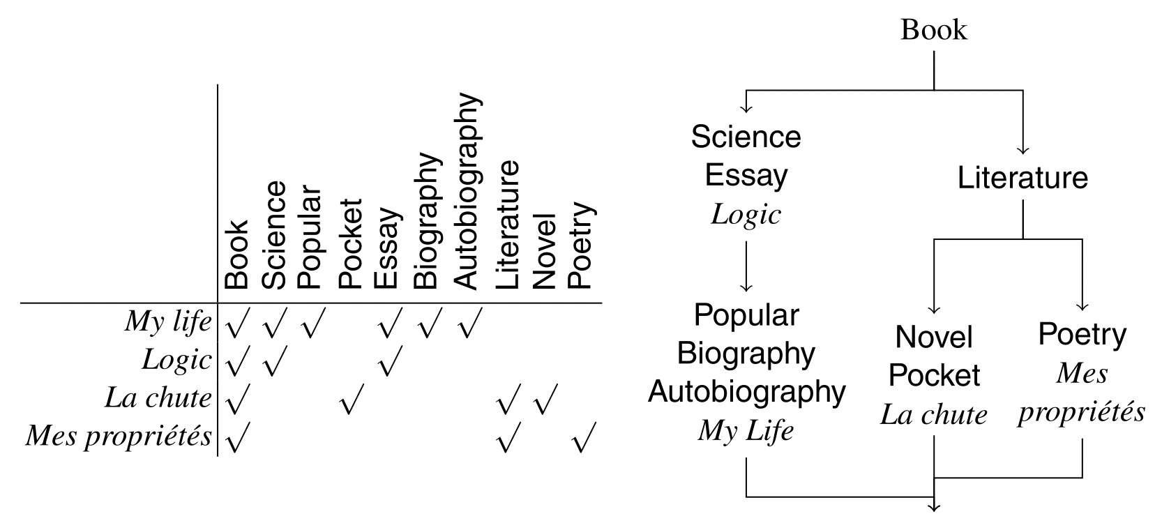
One of the tools of formal concept analysis (FCA) (Ganter and Wille 1999) is the computation of concept lattices. The idea behind formal concept analysis is the duality between a set of objects (in this case, individuals) and their properties. Thus, the set of objects with properties can be organized into a lattice of concepts that cover these objects. Each concept is identified by its properties (intentions) and covers the individuals (scope) that satisfy those properties.
In ontology matching, a property simply needs to be a class to which the indivisual is known to belong, and the method does not depend on the origin of the entity, i.e., whether it comes from the same ontology or not. From this data set, formal concept analysis calculates a concept lattice (or Galois lattice). This is done by computing the closure of the Galois connection of the instance x property. This operation starts with a complete lattice of extent powersets and keeps only the nodes that are closed under the connection. That is, it starts with a set of properties and determines the corresponding set of individuals, which itself provides the corresponding set of properties. If this set is the initial one, it is kept because it is closed, otherwise the node is discarded. As a result, a concept lattice is obtained.

In the table above, a small set of instances and the classes they belong to (from both ontologies) are displayed. On the right side of the figure above, a lattice of corresponding concepts is displayed. From this lattice, the following correspondences can be extracted.

These results are not exact. However, it is possible to weight these results by first eliminating redundant correspondences and then assigning a confidence level based on the size of the area covered by the correspondence.
Techniques for Instance Identification
If there is no common set of instances, it is possible to try to identify which instance of one set corresponds to which instance of the other set. This method becomes effective when the instances are known to be the same. For example, it works well for merging two human resource databases of the same company, but it cannot be applied to databases of different companies or unrelated events.
Such an approach has recently received much attention with the advent of linked data. Indeed, interlinking of data is an important task in linked data (Köpcke and Rahm 2010; Ferrara et al. 2011b), and many algorithms have been redeveloped. Ontology matching can benefit from the retrieval of potential links at the instance level using correspondences (Nikolov et al. 2009; Scharffe and Euzenat 2011). On the other hand, links generated by interlinking of data provide an opportunity to identify instances of matching ontologies. Thus, matchers have been developed that use links from the web of data. This becomes a feedback loop where better alignment provides better linked data, which in turn provides better alignment. The following is a description of such a technique.
Extraction of Link Keys
The first natural way to identify instances is to use the keys of the dataset. There are two types of keys: those that exist inside the dataset, i.e., those for which unique surrogates have been generated (in this case, they are not very useful for identification), and those that exist outside (in this case, they may exist even if these identification keys are not present as keys in both datasets). In such cases, if they are used as keys, they can uniquely identify an individual (as in isbn).
In general, what is really required is what is called a link key. That is, for a pair of classes, it is a set of properties of both ontologies that identifies a pair of instances describing the same individual. The link key should unambiguously identify the entities in both datasets. That is, it should provide a correspondence between the properties of both datasets in order to identify instances with the same value. It must also be unambiguous only for the instances selected by the correspondence, and the key must exist only for these sets.

The key for the bookstore is {isbn},{title,first name},{title,last name}, and for the library data source it is {orig, translator}.
The link key will be ⟨{title, lastname}, {author, orig}, {title = orig, lastname = author}⟩. In other words, the link key uses the non-minimal key of the bookstore dataset. This is because there is no correspondence for the minimal key {isbn} in the library dataset (and thus no correspondence involving isbn). Even more surprisingly, the link key does not use a key from the library dataset. This is because (i) there is no corresponding translator property in the bookstore dataset, and (ii) the set of properties used is sufficient to generate the link unambiguously (which is ⟨year = 1822,author = Quincey,orig = Confessions,translator = Baudelaire⟩, which would have been different if the tuple had existed in the library dataset).
It is also possible to set more elaborate link keys like ⟨{title, lastname, lang}, {ttitle, author}, {lastname = author, title = translate(title, lang)}⟩, which is useful when the orig column is not available. This is useful when orig columns are not available. Such a link key can be useful when unit conversions are needed.
As you can see from this example, the third element of the link key is literally an alignment between properties. In principle, the extraction of keys is done by an algebraic technique that isolates the smallest subset of properties for which no two instances have the same value. Similarly, linked keys can be handled by considering the correspondence (equivalence) between properties and replacing instances by pairs of instances. However, given that linked datasets are open and often of incomplete quality, it would be useful to develop techniques to find keys that maximize the superports that we have in the dataset (Atencia et al. 2012b). Another issue when dealing with ontology expansion becomes the definition of keys when a property or relation has multiple values.
Instance matching based on similarity
In cases where keys do not exist or are different, one approach is to use instance data to compare property values and determine the correspondence between properties. In databases, this technique is known as record linkage (Fellegi and Sunter 1969; Elfeky et al. 2002) or object identification (Lim et al. 1993). These techniques are aimed at identifying multiple representations of the same object in a set of objects. They are usually based on string-based and internal structure-based techniques.
Most of the data interlinkers that deal with instances that cannot be identified by a key operate on the same schema (Ngomo and Auer 2011; Araújo et al. Silk (Section. 12.4.2)), and frameworks such as these describe these two steps exactly. A framework such as Silk (Section. 12.4.2) can accurately describe these two steps. This framework provides a language for plugging in and aggregating similarity measures. The similarity measures to be considered will typically be those considered in this chapter. In addition, measures specific to the type of data to be considered have also been developed, for example, measures for matching geographic areas and addresses.
Since data is usually described by ontologies, classes are the relevant first-level blocks. Therefore, some data interlinkers, such as KnoFuss (Section 12.4.1), can take as input an alignment of ontologies that constrain the classes whose instances are to be compared.
Finally, given that the size of the linked data is usually larger than the size of the ontology, similarity learning becomes more important for two reasons.
– The larger size of the data makes it more difficult to explore the data to select the best approach, and more work needs to be done after the training samples have been extracted.
– Regularity of the data facilitates the efficiency of machine learning.
Therefore, it is not surprising that learning methods such as genetic programming (Section.7.6.2) have been used to interlink data (Ngomo 2011; Isele and Bizer 2013). When the values are not exactly the same, but their distributions can be compared, it is possible to apply global methods. This case is taken up in the next section.
Comparing Disjoint Extensions
When it is not possible to directly infer the data sets common to both ontologies, it is easier to use approximate techniques for comparing class extensions. These techniques can be based on statistical measures of the characteristics of class members, on similarities computed between instances of a class, or on matching between sets of entities.
Statistical approach
Instance data can be used to compute statistics about the property values found in the instances, such as maximum, minimum, average, variance, presence of null values, presence of decimals, scale, precision, grouping, and number of segments. This allows us to characterize the domain of properties of a class from the data. In practice, when dealing with statistically representative samples, these measures should be the same for two equivalent classes of different ontologies.
Consider an example of statistical matching, two ontologies with instances. If we analyze the numerical properties size and weight of one ontology and the numerical properties hauteur and poids of the other, we find that their mean values are different, but their coefficients of variation are the same. The ratio of the mean values of size/hauteur is 2.54 and the ratio of the mean values of weight/poids is 28.35. This is a common phenomenon when the values are expressed in different units.
These values are set based on the entire population. These values can be used to compare the statistical properties of these properties in the classes of the ontology. For example, the average value of the size property of the Pocket class is very different from that of the whole population, and when divided by 28.35, it is very close to that of the Livredepoche class (which is also different from the whole population). Thus, the two classes can be considered similar.
Other approaches (Li and Clifton 1994) use patterns or distributions of data instead of values or domains of data. This results in better fault tolerance and consumes less time because only a small portion of the data values are needed due to the use of data sampling techniques. In general, the application of internal structure methods to instances provides a more accurate picture of the actual structure of the schema elements, and the corresponding data types can be determined more accurately based on the range of values and character patterns found.
However, there is one prerequisite for these methods. That would be that they work well when the correlation between properties is known (otherwise, different properties can be matched based on the domain). This would already be a matching problem to be solved.
Comparing Extensions Based on Similarity
Similarity-based methods can also be applied when the classes share the same set of instances. In particular, a method based on common extension always returns 0, ignoring the distance between elements of the set, if the two classes do not share an instance. In some cases, it may be desirable to compare sets of instances. This requires a (dis)similarity measure between the instances, which can be obtained by other basic methods.
In data analysis, the linkage aggregation method evaluates the distance between two sets of objects that are only similar. This allows two classes to be compared on the basis of their instances.
Definition 40 (Single linkage)
Given a dissimilarity function δ : E × E → R,
the single linkage measure between two sets is the dissimilarity function
 δ : 2E × 2E → Rsuch that∀x,y⊆E,δ(x,y)=min(e,e′)∈x×yδ(e,e′).
Definition 42 (Average linkage)
Given a dissimilarity function δ : E × E → R,
the average linkage measure between two sets is
the dissimilarity function δ : 2E ×
Other linking methods have also been defined. Each of these methods has its own advantages, for example, maximizing the shortest distance, minimizing the longest distance, and minimizing the average distance. Another method in the same family is the Hausdorff dis-tance, which measures the maximum distance from one set to the nearest point of another set (Hausdorff 1914).
Definition 43 (Hausdorff distance)
For a given dissimilar function δ : E × E → R,
the Hausdorff distance between two sets is
the dissimilar function δ : 2E × 2E → R such that ∀x, y ⊆ E.
\[\Delta(x,y)=max\left(\max_{e\in x}\min_{e’\in y}\delta(e,e’),\max_{e’\in y}\min_{e\in x}\delta(e,e’) \right)\]
Matching-based comparison
The problem with the former distance, but the average, is that its value is a function of the distance between one pair of members of the set. The average linkage, on the other hand, has its value as a function of the distance between all possible comparisons.
In matching-based comparison (Valtchev 1999), the elements to be compared are considered to correspond to each other, i.e., to be the most similar.
Therefore, the distance between the two sets is considered as the value to be minimized, and its computation is an optimization problem, i.e., finding the elements that correspond to each other in both sets. Specifically, it is equivalent to solving a bipartite graph matching problem.
Definition 44 (Match-based similarity)
Given a similarity function σ : E × E → R,
the match-based similarity between two subsets of E is
the similarity function MSim:2E × 2E → Rsuch that ∀x,y⊆ E.
\[MSim(x,y)=\frac{max_{p\in Pairings(x,y)}\left(\sum_{<n,n’>\in p}\sigma(n,n’)\right)}{max(|x|,|y|)}\]
Pairings(x,y) will be a set of mappings from elements of x to elements of y.
This match-based similarity requires that the alignments have already been computed. It also depends on the type of alignment that is required. In fact, the results will vary depending on whether the alignment is required to be injectable or not. Match-based comparisons can also be used to compare sequences (Valtchev 1999).
Summary of techniques for using extended information
Extended information is very important for ontology matching because it provides information that is independent of the conceptual part of the ontology. In fact, an ontology is a way of looking at the world, which is why there are many different ontologies for the same topic (and why they have to be matched). It is believed that extended information has less variability and can be used to match classes exactly.
A very favorable case would be when the two ontologies to be matched share the same instance, or when the instances can be easily connected. This makes it easy to compare the overlap between the two classes. In most situations, however, the instance spaces will be different. In such cases, it is possible to either match these instances to go back to the previous case, or to use purely statistical methods to compare the classes with a global measure for their extension.
Summary of Matching Techniques
We have described the basic techniques that can be used to build correspondences based on terminology (Section 5.2), internal structure (Section 5.3), and extension theory (Section 5.4). This categorization of techniques is natural because each of them deals with a partial view of the ontology.
In order to make use of these technologies, it is crucial to finally propose a panorama of the most used technologies so far, and to indicate the directions in which they can be used. In each direction, much work still needs to be done to find a better way.
In general, these techniques are not used in isolation. They can form the basis of a more global approach or be combined to enhance their respective strengths. This will be the subject of the next section and beyond.

コメント