Boltzmann Distribution
The Boltzmann distribution (Boltzmann distribution) is one of the most important probability distributions in statistical mechanics and physics, which describes how the states of a system are distributed in energy. In particular, in statistical mechanics, this distribution is used to determine the probability distribution of the energy states of a system.
The Boltzmann distribution, named after Ludwig Boltzmann, is generally expressed as follows for the probability \(P_i\) of a state \(i\) with energy \(E_i\).
\[ P_i = \frac{e^{-\beta E_i}}{Z} \]
where \(e\) is the base of the natural logarithm, \(\beta\) is the inverse temperature \(1/kT\), \(k\) is Boltzmann’s constant and \(T\) is the absolute temperature, and \(Z\) is called the partition function.
\[ Z = \sum_{i} e^{-\beta E_i} \]
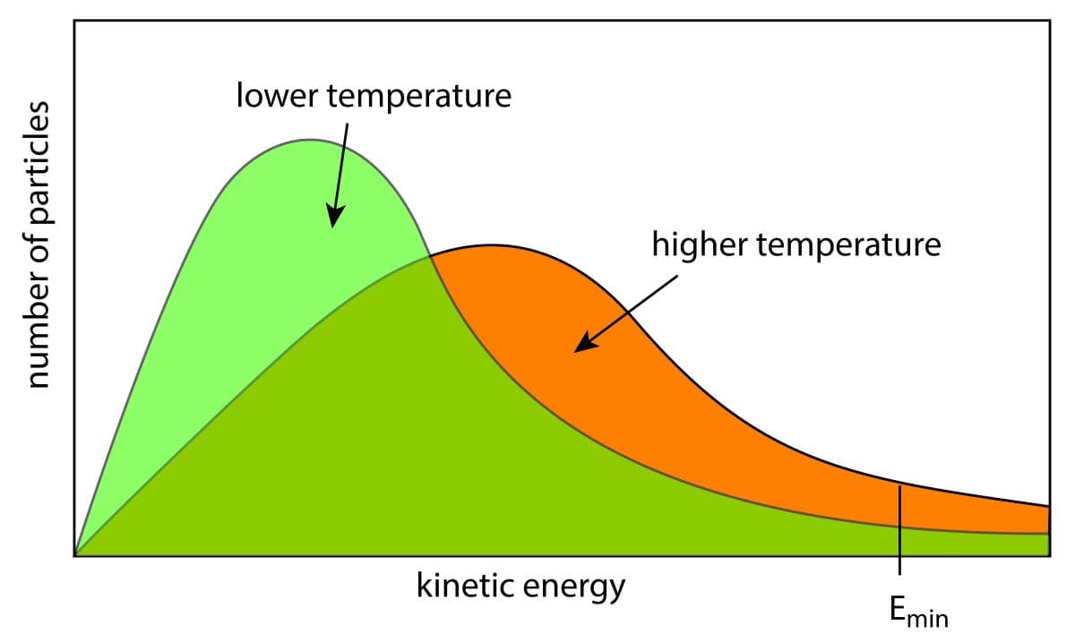
This distribution represents the probability of the system being in each energy state \(E_i\) when the system is in equilibrium, and as can be seen from the Boltzmann distribution, the system tends to be more probable in the lower energy states and less probable in the higher energy states.

The Boltzmann distribution is an indispensable tool for understanding thermodynamic properties of materials, states of matter, phase transitions, etc. For example, the Boltzmann distribution is used to know the probability distribution of energy states inside solids, liquids and gases.
The Boltzmann distribution has also been applied to machine learning and optimization algorithms. For example, the optimization method called simulated annealing uses the Boltzmann distribution to search for optimal solutions. The role of the Boltzmann distribution in machine learning is described below.
Boltzmann distribution and its relationship to machine learning and optimization algorithms
The Boltzmann distribution is one of the probability distributions that play an important role in machine learning and optimization algorithms, especially in stochastic approaches and Monte Carlo based methods with a wide range of applications as follows
1. model learning and probabilistic approaches:
In machine learning, stochastic treatment of data and parameters is common in model learning. For example, Stochastic Gradient Descent (SGD) is a type of optimization algorithm that uses random samples to update the parameters of a model to The gradient is estimated. The Boltzmann distribution plays an important role in learning methods based on stochastic approaches, such as models with stochastic variables that follow the Boltzmann distribution and models called Boltzmann machines, which are also discussed in “Graphical Model Examples. These models use probabilistic learning algorithms to learn parameters and capture patterns in the data.

2. Monte Carlo methods:
The Boltzmann distribution also plays an important role in Monte Carlo methods. For example, a sampling method based on the Boltzmann distribution is the Markov Chain Monte Carlo (MCMC) method described in “Overview and Implementation of Markov Chain Monte Carlo Methods. MCMC is used to study the properties of probability distributions and to solve optimization problems by generating samples that follow the Boltzmann distribution.
3. simulated annealing:
The Boltzmann distribution is also used in an optimization technique called Simulated Annealing. Simulated annealing is a technique that mimics physical annealing (the process of preparing crystals by heating and gradually cooling a metal) and is used to solve optimization problems. In this method, the Boltzmann distribution is used to define the probability of state transitions in the search space, and simulated annealing searches for the optimal solution by setting an initial temperature and then gradually decreasing that temperature while performing a stochastic search based on the Boltzmann distribution.
4. energy minimization:
The Boltzmann distribution is also used in energy minimization problems. For example, energy corresponds to the state of the system, and the Boltzmann distribution can be thought of as giving the probability of the state of the system, so that the state with the highest probability, i.e., the state with the minimum energy, can be found.
Softmax Algorithm
The Softmax Algorithm, also described in “Overview of Softmax Function, Related Algorithms and Examples of Implementation,” is an algorithm for calculating the probability distribution of classes in a multi-class classification problem and is widely used mainly in the fields of machine learning and neural networks. It is widely used in machine learning and neural networks.
In multi-class classification problems, it is necessary to predict which class a given input data belongs to, and the Softmax Algorithm is often used in the output layer of neural networks to obtain the probability distribution for each class.
In addition, a parameter called the temperature parameter plays an important role in this algorithm, and the temperature parameter is used to control the behavior of the softmax function.
To consider them, we first look back at the softmax function. The softmax function for \(K\) different values \(z_1, z_2, … , z_K\) are defined as follows.
\[ \text{Softmax}(z_i) = \frac{e^{z_i}}{\sum_{j=1}^{K} e^{z_j}} \]
where \(e\) is the Napier number (the base of the natural logarithm) and \(z_i\) is the \(i\)th component of the input. The function calculates the probability distribution of each input by computing the exponential function of the input and dividing it by the sum of the exponential functions of all the inputs. In this case, \(z_i\) can be thought of as the “energy” belonging to each class \(i\).
Introducing a temperature parameter \(T\) into this function, the softmax function can be transformed as follows.
\[ \text{Softmax}(z_i) = \frac{e^{z_i/T}}{\sum_{j=1}^{K} e^{z_j/T}} \]
This equation transforms \(z_i\) into a value divided by \(T\), where the temperature parameter \(T\) affects the output of the softmax function and adjusts the “flatness” of the probability distribution.
Transformed in this way, the softmax algorithm can be viewed as a generalization of the Boltzmann distribution described above, and the softmax algorithm can be applied to machine learning approaches where the Boltzmann distribution has been applied as described above.
The application of the softmax algorithm to the bandit problem is described in detail below.
Bandit Problem and Softmax Algorithm
The Multi-armed Bandit Problem (MBA) is a typical problem dealing with the trade-off between search and exploitation, where there are multiple alternatives (bandit arms) and the reward distribution for each alternative is unknown, and the decision of which alternative to choose is the one that will ultimately yield the highest reward Obtaining the highest reward is the approach to solving the target task.
The softmax algorithm is used to solve this bandit problem. The softmax algorithm allows the selection probabilities to be calculated based on the expected reward of each bandit arm, and the bandit arm can be selected probabilistically. The specific procedure is as follows
1. Estimate the value of each arm: Estimate the expected reward (or value) of each bandit arm \(i\). Let this be \(Q_i\).
2. Calculate the probability of selection by softmax function: Calculate the probability of selection \(p_i\) for each arm \(i\) as follows
\[ p_i = \frac{e^{Q_i / \tau}}{\sum_{j=1}^{k} e^{Q_j / \tau}} \]
where \(\tau\) is the temperature parameter; the higher the temperature, the closer to uniform the selection probability, and the lower the temperature, the higher the probability that the arm with the higher value will be selected.
3. Arm selection: Based on the calculated selection probability, the bandit arm \(i\) is selected probabilistically.
4. Acquiring Reward: Receive reward \(r\) from the selected bandit arm \(i\).
5. Update the value: Update the value \(Q_i\) of the selected arm \(i\). Using the reward \(r\), update as follows
\[ Q_i \leftarrow Q_i + \alpha (r – Q_i) \]
where \(\alpha\) is the learning rate, which adjusts how much it is affected by new information.
6. Iteration: Repeat steps 2. through 5. to select the arm that maximizes the reward.
The temperature parameter \(\tau\) in the softmax algorithm is used to adjust the balance between exploration and exploitation; when the temperature is high (\(\tau\) is large), all options are selected with approximately equal probability, thus promoting exploration and prioritizing exploration to acquire new information. When the temperature is low (\(\tau\) is small), the utilization is promoted because high-value alternatives are selected with high probability, and the goal is to utilize known information and maximize rewards.
Thus, the softmax algorithm can be used to adjust the balance between exploration and utilization by setting the temperature parameters to assist in finding the optimal solution. In practice, the temperature is adjusted to raise the temperature and promote search in the early stages of search, and to lower the temperature and promote utilization as the search progresses.
Example implementation of the softmax algorithm applied to the bandit problem
The following is a simple implementation of the softmax algorithm applied to the Bandit problem using Python.
import numpy as np

class SoftmaxBandit:
    def __init__(self, num_actions, temperature):
        self.num_actions = num_actions
        self.temperature = temperature
        self.action_values = np.zeros(num_actions)
        self.action_counts = np.zeros(num_actions)
        self.total_reward = 0

    def softmax(self, action_values):
        exp_values = np.exp(action_values / self.temperature)
        return exp_values / np.sum(exp_values)

    def select_action(self):
        probabilities = self.softmax(self.action_values)
        action = np.random.choice(self.num_actions, p=probabilities)
        return action

    def update(self, action, reward):
        self.total_reward += reward
        self.action_counts[action] += 1
        self.action_values[action] += (reward - self.action_values[action]) / self.action_counts[action]

# Simulation of the Bandit Problem
def bandit_simulation(num_actions, num_steps, temperature):
    bandit = SoftmaxBandit(num_actions, temperature)
    rewards = []
    for _ in range(num_steps):
        action = bandit.select_action()
        # Set up a temporary reward (in this case, a random reward)
        reward = np.random.normal(loc=0, scale=1)
        bandit.update(action, reward)
        rewards.append(reward)
    return rewards

# Running the simulation
num_actions = 5  # Number of arms
num_steps = 1000  # Number of Steps
temperature = 0.5  # Softmax temperature parameters

rewards = bandit_simulation(num_actions, num_steps, temperature)
print("Total reward:", sum(rewards))
In this code, the SoftmaxBandit class implements the softmax algorithm, the action is selected by the softmax function in the select_action method, and the arm value is updated based on the reward in the update method. bandit_. simulation function simulates the bandit problem and returns the total reward for a specified number of steps. When this code is executed, the total reward obtained during the specified number of steps is displayed.
Challenges and remedies when applying the softmax algorithm to the bandit problem
There are various challenges in applying the softmax algorithm to the bandit problem, and there are corresponding measures to address them. They are described below.
1. temperature parameter selection:
Challenge: The softmax function has a temperature parameter, which controls its impact on the choice of action. The choice of the appropriate temperature parameter is important, as it affects the performance of the algorithm. If the temperature is too high, the selection probability between actions will be almost uniform; if the temperature is too low, the action with the highest reward will almost always be selected.
Solution: The initial values of the temperature parameters could be set and optimal values found through experimentation or simulation, or a method of dynamically adjusting the temperature could be employed.
2. balance between exploration and exploitation:
Challenge: In the bandit problem, it is important to strike a balance between exploration (trying new actions) and exploitation (selecting highly rewarding actions based on past experience). Softmax algorithms use probabilistic methods for exploration, but excessive exploration may prevent maximizing the reward.
Solution: The epsilon-greedy method described in “Overview of the epsilon-greedy method (epsilon-greedy), algorithm, and implementation examples” and the UCB method described in “Overview of the Upper Confidence Bound (UCB) algorithm and implementation examples” can be combined with other search methods to achieve balance. For example, a high search rate can be set in the early stages. For example, a high search rate can be set in the initial stage, and the search rate can be decreased gradually.
3. convergence to a locally optimal solution:
Challenge: The softmax algorithm is stochastic, and even if the selected action is not optimal, it may select another action with a certain probability. This may lead to convergence to a locally optimal solution.
Solution: Convergence to a locally optimal solution can be avoided by adjusting temperature parameters or introducing a dynamic search method. It is also effective to use a combination of multiple algorithms.
Reference Information and Reference Books
More details on the bandit problem are given in “Theory and Algorithms of the Bandit Problem“.
Information on the web includes “Netflix Uses Contextual Bandit Algorithm,” “Contextual Bandit LinUCB LinTS,” “Composition of a Recommender System Using the Bandit Algorithm,” and “Rental Property Search System Using Contextual Bandit. Bandit-based Rental Property Search System“.
A reference book is “Bandit problems: Sequential Allocation of Experiments“.

“Regret Analysis of Stochastic and Nonstochastic Multi-armed Bandit Problems“


コメント