Overview of Stable Diffusion
Stable Diffusion is a method used in the field of machine learning and generative modeling, and is an extension of the Diffusion Models described in “Overview, Algorithms, and Examples of Implementations of Diffusion Models” which are known as generative models for images and audio. Diffusion Models are known for their high performance in image generation and restoration, and Stable Diffusion expands on this to enable higher quality and more stable generation.
Features:
1. High quality generation: Stable Diffusion is capable of producing very high quality results for image and audio generation. This makes it well suited for generating high-resolution images and natural sound.
2. stable learning: Generative models are usually difficult to train stably, but Stable Diffusion, as the name implies, is capable of stable learning, which allows for training high quality models in a shorter amount of time.
3. hierarchical generation: Stable Diffusion can generate images, audio, etc. in a hierarchical manner, which is suitable for generating data with more complex structures.
4. High flexibility: Stable Diffusion is flexible enough to handle a variety of data formats and can be used to generate different types of data, such as images, audio, and text.
Algorithms related to Stable Diffusion
The following is an overview of the Stable Diffusion algorithm:
1. Diffusion Process: In the first step, a “diffusion process” is initiated in which the input image is gradually contaminated with noise. This can be thought of as the initialization phase of the image to be generated.
2. Sampling: At each step of the diffusion process, some pixels are sampled as the noise gradually increases. These sampled pixels are the source of information for restoration in the next step.
3. Restoration: The image is reconstructed based on the sampled pixels. This is done by proceeding in the opposite direction of the diffusion process, where the restoration process estimates the surrounding pixels around the sampled pixel.
4. Reconstruction: The final generated image is constructed by combining the results of the diffusion and restoration processes. In this stage, the recovered pixels are combined with information from the original image to produce the final output.
Stable Diffusion Application Examples
Stable Diffusion has been widely applied in various fields such as image creation, image restoration, and image editing. The following are examples of such applications.
1. Image Generation: Stable Diffusion is known to provide more stable and higher quality image generation compared to GANs (Generative Adversarial Networks). It is useful for natural image generation, especially for high-resolution image generation, which makes it suitable for use in artistic creative activities and the design industry.
2. Image Restoration: Stable Diffusion is also used to repair damaged images and fill in missing areas. Stable Diffusion can effectively remove damage and noise while maintaining the natural look of the restored image.
3. Image Editing: Stable Diffusion can also be used to edit specific areas of an image. For example, faces and backgrounds can be modified, unwanted objects can be removed, and images can be restyled.
4. Domain Adaptation: Stable Diffusion is also used for image transformation between different domains and domain adaptation. Examples include converting daytime images to nighttime images, or photographs to art style, which is useful when sensor data needs to be converted or synthesized in domains such as automated driving technology or robotics.
Utilization and implementation of Stable Diffusion
Stable Diffusion is available through three web services: Hugging Face, Dream Studio, and Mage.
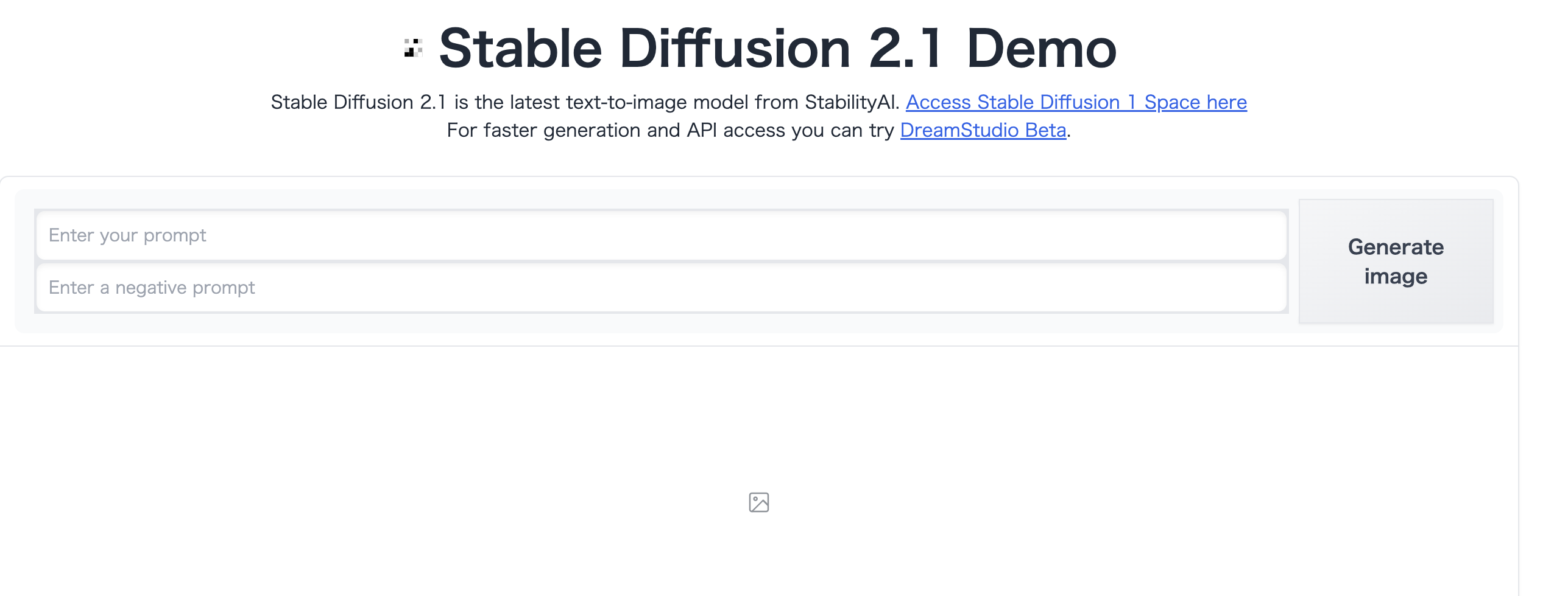
Hugging Face, described in “Overview of Automatic Sentence Generation with Huggingface,” is a repository of generative models and includes the “Stable Diffusion 2 Demo,” a demonstration of Stable Diffusion.

The operational procedure for using Stable Diffusion 2 is very simple: simply enter the text representing the image you wish to generate in the text input area and click the Execute Image Generation button. The generated image shall be the one displayed.
You can also download and run AUTOMATIC’s stable-diffusion-webui as described in “Codeless Generation Module Using text-generation-webui and AUTOMATIC1111” to launch a web version of stable You can also launch a web version of stable-diffusion locally by downloading and running AUTOMATIC’s stable-diffusion-webui.

Example of Fine Tuning Implementation with LoRA by Stable Diffusion
Stable Diffusion fine tuning can be performed using LoRA, as described in “Overview of LLM Fine Tuning with LoRA and Example Implementation“. Specifically, the following procedure is used to perform LoRA fine tuning using PyTorch.
Prepare a Stable Diffusion model: First, prepare the original Stable Diffusion model. This model should be pre-trained for tasks such as generation, repair, and editing.
LoRA Preparation: Next, the LoRA implementation is prepared in PyTorch. This includes the network architecture and training process of LoRA, and can be done by referring to the official LoRA repository and related research papers.
Fine Tuning Setup: Setup for fine tuning. In this case, load the Stable Diffusion model and apply LoRA’s optimization methods. Also, configure the dataset and training parameters for fine tuning.
Perform fine tuning: Based on the above settings, LoRA is applied to the Stable Diffusion model to perform fine tuning. Iteratively train the model using the training dataset.
Evaluate and analyze results: Once fine tuning is complete, evaluate the performance of the model using the evaluation dataset and analyze the results. Evaluate the quality of the generated images and the accuracy of the repaired images.
The following is a simple example of fine tuning Stable Diffusion with LoRA using Python and PyTorch.
import torch
import torch.optim as optim
from stable_diffusion_model import StableDiffusionModel
from lora_model import LoRAModel
from dataset import CustomDataset
from torch.utils.data import DataLoader

# Loading Stable Diffusion Models
sd_model = StableDiffusionModel()
sd_model.load_state_dict(torch.load('sd_model.pth'))
sd_model.eval()

# LoRA Model Preparation
lora_model = LoRAModel()
optimizer = optim.Adam(lora_model.parameters(), lr=0.001)

# Prepare dataset and data loader for fine tuning
dataset = CustomDataset(...)
dataloader = DataLoader(dataset, batch_size=32, shuffle=True)

# Perform fine tuning
for epoch in range(num_epochs):
    for data in dataloader:
        inputs, targets = data
        optimizer.zero_grad()
        outputs = lora_model(sd_model(inputs))
        loss = compute_loss(outputs, targets)  # Calculation of Loss Functions
        loss.backward()
        optimizer.step()

# Saving the model after fine tuning
torch.save(lora_model.state_dict(), 'finetuned_lora_model.pth')
This code shows the basic procedure for fine tuning using a combination of the Stable Diffusion and LoRA models.
For more detailed applications, see also “What is LoRA (LoRA)|Trying Fine Tuning of This Year’s Hot Image Generation AI (Stable Diffusion),” “[Stable Diffusion Web UI] How to Use the Additional Learning Model LoRA,” and “What is LoRA? What is LoRA?“.
Challenges of Stable Diffusion and how to deal with them
Stable Diffusion is a powerful image generation and restoration method, but there are some challenges. The challenges and their solutions are described below. 1.
1. high computational load:
Challenge: Stable Diffusion can be computationally very expensive, especially for high-resolution images and large datasets, and training and inference can be slow.
Solution: Use high-performance hardware and distributed training to increase computational speed. Optimize network architecture to reduce model complexity. Consider alternative lightweight methods and models.
2. dependence on data diversity:
Challenge: The performance of Stable Diffusion is dependent on the diversity of the dataset used for training. If there is a bias toward a particular dataset, the model may not be generalizable.
Solution: Collect data from multiple data sources to ensure diversity in training data. Use data augmentation techniques to increase training data variation. Adapt models to data from other domains using techniques such as domain adaptation and transfer learning.
3. improve quality of generated images:
Challenge: There is room for improvement in the quality of images produced by Stable Diffusion, especially under certain conditions where unnatural artifacts and missing details can be problematic.
Solution: Adjust the model’s loss function to improve the quality of the generated images. Adjust the model’s architecture to capture more complex features. Explore and combine alternative approaches and methods for image generation.
4. limitation of handling noise and missing features:
Challenge: Stable Diffusion is effective in handling noise and missing features, but has limitations under certain conditions. For example, in the case of large missing areas or extreme noise, adequate restoration may be difficult.
Solution: Apply appropriate preprocessing or data enhancement techniques depending on the pattern of noise or missing data. Use appropriate loss functions and model architecture to reflect noise and missing patterns in the model. etc. are possible.
Reference Information and Reference Books
For details on image information processing, see “Image Information Processing Techniques.
Reference book is “

“

“

“


コメント