Overview of PATCHY-SAN
The Spectral Graph Convolutional Neural Networks (GCN) described in “Overview, Algorithm and Implementation Examples of Graph Convolutional Neural Networks (GCN)” and “Overview, Algorithm and Implementation Examples of ChebNet” had the following issues. Convolutionalization had the following issues.
Computational explosion when the graph is large, since eigenvalues are calculated from adjacency matrices and the entire graph is handled.
Spectral graph convolution assumes that the graph structure is fixed, so it is difficult to generalize to different graphs, and the learned filter cannot be applied to other structures.
Since the definition of the graph Laplacian for directed graphs is not well defined, Spectral graph convolution can only handle undirected graphs. Any variation on the graph will cause variation on the underlying eigenvectors.
Spectral graph convolution is a graph signal processing standpoint, and to improve them, Spacial graph convolution, which reflects the graph structure by using and updating the representation of surrounding nodes when learning the representation of a node, is being considered.
In this article, we describe PATCHY-SAN, one such spacial graph convolution.
PATCHY-SAN was proposed by Niepert in “Learning Convolutional Neural Networks for Graphs,” and it addresses two problems in graph convolution: determining the sequence of nodes that form a neighborhood graph and computing the normalization of the neighborhood graph. The proposed method solves these problems for arbitrary graphs.
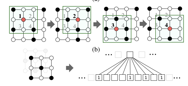
This method uses the Weisfeiler-Lehman (WL) kernel, a graph kernel, to measure the similarity between graphs. The specific steps are (1) first sort the nodes by the labels attached by the WL kernel, select a certain number (ω) of nodes from the graph, select k nodes that are close in distance to it, and order them to obtain a matrix, (2) repeat this for each attribute (a_v) of a node to obtain ( (2) Repeat this process for each node attribute (a_v) to create a tensor of ( omegatimes ktimes a_v), and (3) Perform convolution based on this tensor in the same way as for an image.

With this approach, PATCHT-SAN has the following three characteristics
- The computational complexity is nearly linear with respect to the number of nodes, making it applicable to large graphs.

The table above will show the processing time between PATCHT-SAN and conventional GCN. In the conventional method, the processing time increases as the size of the graph increases, but in PATCHT-SAN, the processing time is significantly reduced.
- It has the ability to visualize the learned features and thereby find the structure of the graph.

The above figures are the result of visualization with a restricted Boltzmann machine (RBM). Instances of these graphs of about 100 nodes for a torus (top left), a preferential attachment graph (bottom left), a co-purchasing network of political books (top right), and a random graph (bottom right) are depicted on the left side respectively, are depicted on the left. Also shown is a visual representation of the weights of the features (the darker the color of the pixel, the stronger the corresponding weight) and three graphs sampled from the RBM with all but the hidden nodes corresponding to the features set. The yellow node here is the one with position 1 in the adjacency matrix.
- It is possible to learn features that depend on the target region without having to manually build up the features.
Algorithm of PATCHY-SAN
The basic algorithm of PATCHY-SAN is shown below. (Excerpt from “Learning Convolutional Neural Networks for Graphs”)
1. Select Node Sequence:
Selection of a node sequence is the selection of a receptor sequence for each input graph. Algorithm 1 is one such procedure.
First, the vertices of the input graph are sorted with respect to the given graph label. Next, the resulting node sequence is traversed at a given stride s. For each node visited, the algorithm shall be executed and receptive fields shall be constructed until exactly w receptive fields are created.
1: input: graph labeling procedure `, graph G = (V, E), stride
s, width w, receptive field size k
2: Vsort = top w elements of V according to `
3: i = 1, j = 1
4: while j < w do
5: if i ≤ |Vsort| then
6: f = RECEPTIVEFIELD(Vsort[i])
7: else
8: f = ZERORECEPTIVEFIELD()
9: apply f to each input channel
10: i = i + s, j = j + 1
2. Neighborhood Assembly:
For each node identified in the previous step, a local neighborhood of the input node is constructed to construct the receptive field. The nodes in the neighborhood are candidates for receptive fields. Given node v and receptive field size k as input, this procedure performs a width-first search, searching for vertices with increasing distance from v. If the number of nodes collected is less than k, one neighborhood of the most recently added vertex in N is collected, and at least k vertices are in N or, The search shall continue until there are no more neighborhoods to add.
1: input: vertex v, receptive field size k
2: output: set of neighborhood nodes N for v
3: N = [v]
4: L = [v]
5: while |N| < k and |L| > 0 do
6: L =
S
v∈L N1(v)
7: N = N ∪ L
8: return the set of vertices N
3. Create Receptive Field:
1: input: vertex v, graph labeling `, receptive field size k
2: N = NEIGHASSEMB(v, k)
3: Gnorm = NORMALIZEGRAPH(N, v, `, k)
4: return Gnorm
4. Graph Normalization:
The receptive field of nodes is constructed by normalizing the neighborhood assembled in the previous step. The normalization gives an order to the nodes in the neighborhood graph, mapping them from an unordered graph space to a linearly ordered vector space. The basic idea is to utilize a graph labeling procedure that assigns the nodes of two different graphs to similar relative positions in their respective neighborhood matrices, provided that the structural roles in the graphs are similar.
1: input: subset of vertices U from original graph G, vertex v,
graph labeling `, receptive field size k
2: output: receptive field for v
3: compute ranking r of U using `, subject to
∀u, w ∈ U : d(u, v) < d(w, v) ⇒ r(u) < r(w) 4: if |U| > k then
5: N = top k vertices in U according to r
6: compute ranking r of N using `, subject to
∀u, w ∈ N : d(u, v) < d(w, v) ⇒ r(u) < r(w)
7: else if |V | < k then
8: N = U and k − |U| dummy nodes
9: else
10: N = U
11: construct the subgraph G[N] for the vertices N
12: canonicalize G[N], respecting the prior coloring r
13: return G[N]
The specific PATCHY-SAN code is available on Niepert’s git page.
Challenge of PATCHY-SAN
Challenges with PATCHY-SAN include the fact that convolution strongly depends on graph labeling (which is pre-processing, not learning) and that ordering the nodes in one dimension is not a natural choice.
Another issue is that graph labeling considers only the structure of the graph and not the characteristics of the nodes.
Reference Information and Reference Books
For more information on graph data, see “Graph Data Processing Algorithms and Applications to Machine Learning/Artificial Intelligence Tasks. Also see “Knowledge Information Processing Techniques” for details specific to knowledge graphs. For more information on deep learning in general, see “About Deep Learning.
Reference book is

“Graph Neural Networks: Foundations, Frontiers, and Applications“等がある。

“Introduction to Graph Neural Networks“

“Graph Neural Networks in Action“


コメント